Biol20N02 2017 and Monte Carlo Club: Difference between pages
imported>Weigang |
imported>Weigang |
||
| Line 1: | Line 1: | ||
__FORCETOC__ | |||
=Season V. Genes, Memes, and Machines (Spring 2022)= | |||
* A journal club to continue the exploration of the link between evolution & learning. | |||
* [https://pages.cs.wisc.edu/~dyer/cs540/handouts/info-theory-primer.pdf A primer for information theory] | |||
* Data ≠ Information: Scharf (2021). The Ascent of Information: Books, Bits, Genes, Machines, and Life's Unending Algorithms. [https://www.amazon.com/Ascent-Information-Machines-Unending-Algorithm/dp/0593087240 Amazon link] | |||
* The "It's the song not the singer" (ITSNTS) theory of selection unit: [https://pubmed.ncbi.nlm.nih.gov/29581311/ Doolittle & Inkpen (2018).] "Processes and patterns of interaction as units of selection: An introduction to ITSNTS thinking", PNAS. | |||
---- | * Evolution is an AI machine: [https://www.oreilly.com/radar/open-endedness-the-last-grand-challenge-youve-never-heard-of/ Stanley, Lehman, and Soros (2017).] "Open-endedness: The last grand challenge you’ve never heard of - While open-endedness could be a force for discovering intelligence, it could also be a component of AI itself." O'Reily | ||
* An algorithmic definition of individuality: [https://pubmed.ncbi.nlm.nih.gov/32212028/ Krakauer et al (2020)]. "The information theory of individuality". Theory BioSci | |||
* Evolution towards complexification: [https://aip.scitation.org/doi/abs/10.1063/1.3643064 Krakauer (2011)]. "Darwinian demons, evolutionary complexity, and information maximization". Chaos. | |||
=Season IV. Classification using Machine Learning (Summer 2021)= | |||
* Textbook: Aurélien Géron (2019). Hands-On Machine Learning with Scikit-Learn, Keras, and TensorFlow: Concepts, Tools, and Techniques to Build Intelligent Systems, 2nd Edition. [https://www.amazon.com/gp/product/1492032646/ref=ppx_yo_dt_b_asin_title_o00_s00?ie=UTF8&psc=1 Amazon link] | |||
* Set up Python work environment with [https://docs.conda.io/en/latest/miniconda.html mini-conda] | |||
* We will be using Jupyter-notebook (part of mini-codon installation) to share codes | |||
==Week 1. MNIST dataset (Chapter 3)== | |||
# Dataset loading and display (pg 85-87): Jackie, Niemah, and Hannah | |||
# Binary classifier | |||
## Cross-validation (pg 89-90): Roman, etc | |||
## Confusion matrix (pg 90-92): | |||
## Precision and recall (pg 92-97) | |||
## ROC curve (pg. 97-100) | |||
# Multiclass classification (pg 100-108): Brian, etc | |||
== | ==Week 2. K-means clustering (Chapter 9)== | ||
# 2D simulated dataset | |||
# Image recognition | |||
# MNIST dataset | |||
==Week 3. Exercises (pg.275-276, Chapter 9)== | |||
# Exercise 10: Facial recognition (Olivetti faces dataset, with k-means) | |||
# Exercise 11. Facial recognition (semi-supervised learning | |||
== | =Notes on Origin of Life (Spring 2020)= | ||
# [https://journals.plos.org/plosone/article/metrics?id=10.1371/journal.pone.0224552 Attie et al (2019). Genetic Code optimized as a traveling salesman problem] | |||
# [https://itsatcuny.org/calendar/self-organizing-systems-and-the-origin-of-life GC Origin of Life Seminar (2/19/2021)] | |||
# [https://www.cell.com/current-biology/fulltext/S0960-9822(15)00681-8?_returnURL=https%3A%2F%2Flinkinghub.elsevier.com%2Fretrieve%2Fpii%2FS0960982215006818%3Fshowall%3Dtrue Pressman et al (2015). Review: RNA World (ribozyme as origin of genetic code)] | |||
# A perspective: [https://www.nature.com/articles/s42256-020-00278-8 Miikkulainen, R., Forrest, S. A biological perspective on evolutionary computation. Nat Mach Intell 3, 9–15 (2021)] | |||
== | =Season III. Summer 2018 (Theme: Evolutionary Computing)= | ||
==Week 1. Introduction & Motivating Examples== | |||
# Genetic Arts | |||
## [http://picbreeder.org Go to picbreeker website] & evolve using "branch" method | |||
## Evolve 3D art: [http://endlessforms.com Endless Forms] | |||
## CPPN-NEAT Algorithm: Compositional Pattern Producing Networks (CPPNs)-NeuroEvolution of Augmenting Topologies (NEAT); [https://www.ncbi.nlm.nih.gov/pubmed/20964537 PicBreeder paper]; or [http://campbellssite.com/papers/secretan_chi08.pdf a PDF version] | |||
# [https://www.nature.com/articles/s41586-018-0102-6 NeuroEvolution (by DeepMind team)] | |||
# Robotic snake (and other soft robots) | |||
## A controller built with physics laws difficult (too many parameters) | |||
## Simulation with evolutionary computing: | |||
### (Genotype) A list of 13 commands (one for each segment; each being a neural net, with 25 inputs and one output of joint angles) | |||
### (Phenotype) Fitness function: total displacement | |||
### Algorithm: [https://medium.com/@devonfulcher3/the-map-elites-algorithm-finding-optimality-through-diversity-def6dcbc0f5b MAP-Elites]; [https://www.nature.com/articles/nature14422 Nature paper] | |||
### Approach: training with simulated data | |||
# Robotic Knightfish | |||
## [https://www.youtube.com/watch?v=3XjgZbs0t2g Youtube demo] | |||
## Algorithm: [https://en.wikipedia.org/wiki/CMA-ES CMA-ES (Covariance Matrix Adaptation Evolution Strategy)] | |||
### Genotype: 15 variables (sinusoidal wave function or Fourier Series) | |||
### Phenotype/Fitness: speed | |||
## Implementation: DEAP | |||
# Compositional Protein design (CPD) | |||
## Genotype: side-chain configuration determined by [https://www.ncbi.nlm.nih.gov/pubmed/8464064 rotamer library] | |||
## Phenotype/Fitness: Rosetta energy function & functional (e.g., binding affinity) | |||
## Fitness landscape: each node is a protein structure, each edge represent connections/relatedness | |||
# Simulation-based optimization: [http://simopt.org/ Problem Sets] | |||
# Self-evolving software([http://geneticprogramming.com/ Genetic Programming]) | |||
== | ==Week 2. Toy Problem: OneMax Optimization== | ||
=== | # Problem: Create a list of L random bits (0 or 1). Evolve the list until the fitness reaches the maximum value (i.e., contains only 1's) | ||
# | # Neutral Evolution: | ||
# | ## Create a vector of L random bits (e.g, L=20). Hint for creating a random vector of 0's and 1's in R: <code>ind<-sample(c(0,1), prob=c(0.5.0.5), replace=T, size=20)</code>. Biologically, this vector represents a single haploid genome with 20 loci, each with two possible alleles (0 or 1). | ||
* | ## Create a population of N=100 such individuals. Hint: creating a list of vectors in R: <code>pop <- lapply(1:100, function(x){<insert sample() function above>})</code> | ||
* | ## For each generation, each individual reproduces 10 gametes with mutation (with the probability for bit flip: mu = 1/L = 0.1). Hint: write a mutation function that takes an individual as input and outputs a mutated gamete. Use the "broken stick" algorithm to implement mutation rate: <code>cutoff <- runif(1); ifelse(cutoff <= mu, flip-bits, no-flip)</code> | ||
## Take a random sample of N=100 gametes into the next generation & repeat above | |||
## Plot mean, minimum, and maximum fitness over generations | |||
## Plot diversity statistics over generation (including average allelic heterozygosity per locus as well as haplotype heterozygosity). Hint: write two functions for these heterozygosity | |||
# Add natural selection (proportional scheme) | |||
## Individuals reproduce with fitness proportional to the total number of 1's. | |||
## Iterate until a population contains at least one individual with all 1's | |||
## Plot mean, minimum, and maximum fitness over generations | |||
## Plot diversity (expectation: decreasing) | |||
# Add natural selection (tournament scheme) | |||
## Randomly selecting n=5 individuals and allow the fittest one to make gametes | |||
## Plot mean, minimum, and maximum fitness over generations (Expectation: faster optimization) | |||
## Plot diversity (expectation: decreasing fasters) | |||
# Add crossover | |||
## Hint: write a crossover function | |||
## Does it reach optimization faster? | |||
# Code submissions | |||
## [https://github.com/JohnDi0505/MonteCarlo_Simulation-Biostats/blob/master/OneMax%20Optimization.ipynb Python Notebook by John] | |||
## [http://rpubs.com/weigang/407979 R code by Weigang] | |||
## [http://rpubs.com/ChrisNSP/408534 R code by Panlasigui] | |||
## [https://github.com/Inhenn/Toy_Problem_Bio/blob/master/Bio_Toy.ipynb Python Notebook by Yinheng] | |||
## [http://rpubs.com/desiree/409200 RPub by Desiree] | |||
==Week 3. Python & R Packages for evolutionary computation== | |||
* [http://deap.readthedocs.io/en/master/ DEAP: a Python package for Evolutionary Computing] | |||
** Look under [http://deap.readthedocs.io/en/master/examples/index.html Examples] to repeat the OneMax code | |||
* [https://cran.r-project.org/web/packages/GA/vignettes/GA.html GA: An R package for genetic programming] | |||
** Reference 1 (Examples in Section 4). [https://www.jstatsoft.org/v53/i04/ Scrucca, L. (2013) GA: A Package for Genetic Algorithms in R.] | |||
** Reference 2 (for Advanced applications). [https://journal.r-project.org/archive/2017/RJ-2017-008 Scrucca, L. (2017) On some extensions to GA package: hybrid optimisation, parallelisation and islands evolution. ] | |||
** OneMax code & plots (Weigang) | |||
** Example 4.1a. One variable optimization: f(x) = |x| + cos(x) (Muhammad and Desiree) | |||
** Example 4.1b. One variable optimization: f(x) = (x2 + x) cos(x) | |||
** Example 4.2. Two-parameter optimization: f(x;y) = 20 + x^2 + y^2 * 10(cos(2x) + cos(2y)) (Muhammad and Desiree) | |||
** Example 4.3. Curve-fitting: tree growth | |||
** Example 4.7. Constrained optimization: Knapsack Problem | |||
** Example 4.8. Combinatorial optimization: Traveling Salesman Problem (Brian) | |||
** Advanced application 1. Stock portfolio (Hybrid algorithms) | |||
** Advanced application 2. Parallelization | |||
** Advanced application 3. Island model | |||
* Code submissions | |||
** [http://rpubs.com/weigang/410426 rPub for OneMax (by Weigang)] | |||
** One & Two-dimensional functional optimization with GA (by Desiree & Mohamud) : [http://rpubs.com/desireepante/411065 Entropy function] | |||
** [https://github.com/Inhenn/Knapsack-Problem-Using-DEAP/blob/master/DEAP3.ipynb OneMax and Knapsack Problem with DEAP (by Yinheng)] | |||
** Traveling Salesman Problem with GA (by Brian) | |||
==Week 4. Multiplex Problem== | |||
==Week 5. Genetic Programming== | |||
=Season II. Summer 2017 (Theme: Machine Learning)= | |||
==Week 1. Introduction & the backprop algorithm== | |||
[[File:Iris-box3.png|thumbnail]] [[File:Iris-box4.png|thumbnail]] | |||
# Problem: Classification/Clustering/Predication of flower species (a total of 3 possible species in the sample data set) based on four phenotypic traits/measurements | |||
# The "iris" data set: exploratory data analysis with visualization & descriptive statistics: <code>data("iris"); plot()</code>, <code>summary()</code>, <code>qqnorm(); qqline(); hist()</code>; normalization with <code>scale()</code> (Roy) | |||
# Mathematics of backpropagating errors to neural connections (Oliver) | |||
## Objective/optimization function measuring difference between target (<code>t</code>, expected) and neural activity <code>y</code>: <code>G=Sum{t*log(y)+(1-t)log(1-y)}</code> (this is known as the "cross-entropy" error function; the other alternative is "minimal squared error (MSE)"), which has the gradient in the simple form of <code>g=-(t-y)x, where x is the input</code>. The objective function is minimized when weights are updated by the gradient. Error-minimization by MSE has similar effects but harder to calculate. | |||
## Learning algorithm is presented | |||
==Week 2. Traditional approaches to multivariate clustering/classification== | |||
# Dimension reduction with Multidimensional Scaling <code>cmdscale()</code> [http://rpubs.com/meibyderp/281616 Mei's rNoteBook]. | |||
# Dimension reduction with Principal Component Analysis<code>princomp()</code>. [http://rpubs.com/ssipa/281715 Sipa's rNoteBook] | |||
# Multivariate clustering with Hierarchical Clustering <code>hclust()</code> (Saymon) | |||
# Multivariate clustering with k-means <code>kmeans()</code> [http://rpubs.com/roynunez/281963 Roy's rNoteBook] | |||
# Classification based on logistic regression <code>glm()</code>, linear discriminatory analysis <code>lda()</code>, & k-nearest neighbor <code>library(class); knn()</code> (John) | |||
# Modern, non-linear classifiers: Decision Trees (DT), Support Vector Machines (SVM), and Artificial Neural Networks (ANN) (Brian) | |||
==Week 3. Single-neuron classifier== | |||
# Algorithm: [[File:Ml-image-1a.jpg|thumbnail]] | |||
## Read input data with <code>N=150 flowers</code>. Reduce to a matrix <code>x</code> with two traits (use trait 1 & 3) and two species (use rows 51-150, the last two species, skip the first species [easy to separate]) for simplicity. Create a target vector <code>t <- c(rep(0,50),rep(1,50))</code> indicating two species | |||
## Initialize the neuron with two random weights <code>w<-runif(2, 1e-3, 1e-2)</code> and one random bias <code>b<-runif(1)</code> | |||
## Neuron activation with <code>k=2</code> connection weights: <code>a=sum(x[k] * w[k])</code> | |||
## Neuron activity/output: <code>y=1/(1+exp(-a-b))</code> (This logistic function ensures output values are between zero and one) | |||
## Learning rules: learning rate <code>eta=0.1</code>, backpropagate error ("e") to get two updated weights (for individual <code>i</code>, feature <code>k</code>): <code>e[i]=t[i]-y[i]; g[k,i]= -e[i] * x[k,i]; g.bias[i] = -e[i] for bias</code>; Batch update weights & bias: <code>w[k]=w[k] - eta * sum(g[k,i]); b = b - eta * sum(g.bias[i])</code> (same rule for the bias parameter <code>b</code>); Repeat/update for <code>L=1000 epochs (or generations)</code> | |||
## Output: weights and errors for each epoch | |||
# Evaluation: | |||
## Plot changes of weights over epoch | |||
## Use the last weights and bias to predict species | |||
## Compare prediction with target to get accuracy | |||
## Plot scatter plot (x2 vs x1) and add a line using the weights & bias at epoch=1,50,100,200,500, 1000: <code>a=w1*x1 + w2*x2 + b; a=0</code>. The lines should show increasing separation of the two species. | |||
# Code submissions | |||
## Roy: [http://rpubs.com/roynunez/283699 rPubs notebook] | |||
## John: [https://github.com/JohnDi0505/MonteCarlo_Simulation-Biostats/blob/master/Neuron_Networks/Single_Neuron_Classification.py Python code on github] | |||
## Mei: [http://rpubs.com/meibyderp/284498 rPubs notebook] | |||
## Brian: [http://rpubs.com/drtwisto/286938 rPubs notebook] | |||
## Weigang: [http://rpubs.com/weigang/279898 rPubs notebook] | |||
# Questions for future exploration | |||
## How to avoid over-fitting by regularization (a way to penalize model complexity by adding a weight decay parameter <code>alpha</code>) | |||
## Bayesian confidence interval of predictions (with Monte Carlo simulation) | |||
## Limitations: equivalent to PCA (linear combination of features); adding a hidden layer generalize the neural net to be a non-linear classifier | |||
==Week 4. Single-layer, multiple-neuron learner== | |||
[[File:Multiple-neuron-learner.png|thumbnail]] | |||
# Predict all three species (with "one-hot" coding) using all four features: e.g., 100 for species 1, 010 for species 2, and 001 for species 3. Create 3 neurons, each one outputting one digit. | |||
# Use three neurons, each accepts 4 inputs and output 1 activity | |||
# Use softmax to normalize the final three output activities | |||
# Code submissions | |||
## John: | |||
### [http://www.kdnuggets.com/2016/07/softmax-regression-related-logistic-regression.html reference this webpage] | |||
### [https://github.com/JohnDi0505/MonteCarlo_Simulation-Biostats/blob/master/Neuron_Networks/Multiple_Neuron_Classification.py Python code] | |||
### TensorFlow code | |||
## Roy: [http://rpubs.com/roynunez/288023 rpubs notebook] | |||
## Mei: [http://rpubs.com/meibyderp/288400 rPubs Notebook] | |||
## Weigang: [http://rpubs.com/weigang/287025 rPubs notebook] | |||
# Challenge: Implementation with TensorFlow, an Open Source python machine learning library by Google Deep Mind team. Follow [https://www.tensorflow.org/get_started/mnist/beginners this example of softmax regression] | |||
# A biological application for the summer: identify SNPs associated with biofilm/swarming behavior in Pseudomonas | |||
==Week 5. Multi-layer ("Deep") Neuron Network== | |||
[[File:Iris-nnet.png|thumbnail]] | |||
[[File:Nnet-overfitting.png|thumbnail|An investigation of under-fitting (at N=1) & over-fitting (at N=3 nodes). N=0 implies linear fitting.]] | |||
# Input layer: 4 nodes (one for each feature) | |||
# Output layer: 3 nodes (one for each species) | |||
# Hidden layer: 2 hidden nodes | |||
# Advantage: allows non-linear classification; using hidden layers ("convoluted neural net") is able to capture high-order patterns | |||
# Implementation: I'm not going to hard-code the algorithm from scratch. The figure was produced using the R package with the following code: <code>library(nnet); library(neuralnet); targets.nn <- class.ind(c(rep("setosa",50), rep("versicolor",50), rep("virginica",50))) # 1-of-N encoding; iris.net <- neuralnet(formula = setosa + versicolor + virginica ~ Sepal.Length + Sepal.Width + Petal.Length + Petal.Width, data = training.iris, hidden = 2, threshold = 0.01, linear.output = T); plot(iris.net, rep="best")</code>. It achieved 98.0% accuracy. | |||
# Deep neural net allows non-linear, better fitting, but we don't want over-fitting by adding more hidden layers (or more neurons in the hidden layer). Identify under- and over-fitting with the following procedure: | |||
## Randomly sample 100 as training set and the remaining as target. Repeat 100 times | |||
## For each sample, plot accuracy for the training set, as well as accuracy for the target | |||
## Find the point with the right balance of under- and over-fitting | |||
==Week 6. Unsupervised Neural Learner: Hopfield Networks== | |||
# Hebbian model of memory formation (MacKay, Chapter 42). Preparatory work: | |||
## Construct four memories, each for a letter ("D", "J", "C", and "M") using a 5-by-5 grid, with "-1" indicating blank space, and "1" indicating a pixel. Flatten the 5-by-5 matrix to a one-dimensional 1-by-25 vector (tensor). | |||
## Write two functions, one to show a letter <code>show.letter(letter.vector)</code>, which draws a pixel art of letters (print a blank if if -1, a "x" if 1), another to mutate the letter <code>mutate(letter.vector, number.pixel.flips)</code> | |||
# [https://en.wikipedia.org/wiki/Hopfield_network Hopfield Network] | |||
## Store the four memories into a weight matrix, which consists of symmetric weights between neurons i and neuron j, i.e., w[i,j] = w[j,i]. We will use a total of 25 neurons, one for each pixel. | |||
## First, combine the four vectors (one for each letter) into a matrix: <code>x <- matrix(c(letter.d, letter.j, letter.c, letter.m), nrow = 4, byrow = T)</code> | |||
## Second, calculate weight matrix by obtaining the outer product of a matrix multiplication: <code>w <- t(x) %*% x</code>. Set diagonal values to be all 0's (i.e., to remove all self-connections): <code>for (i in 1:25) { w[i,i] = 0 }</code>. This implements [https://en.wikipedia.org/wiki/Hebbian_theory Hebb learning], which translates correlations into strength of connections quantified by weights: large positive weights indicate mutual stimulation (e.g., 1 * 1 = 1 [to wire/strengthen the connection of co-firing neurons, and ...], -1 * -1 = 1 [to wire/strengthen the connection of co-inhibitory neurons as well]), large negative weights indicate mutual inhibition (e.g., 1 * -1 = -1 [to unwire/disconnect oppositely activated neurons]), and small weights indicate a weak connection (e.g., 0 * 1 = 0 [to weaken connections between neurons with uncorrelated activities, but do not unwire them]). (0, 1, and -1 being values of neuron activities) | |||
## Third, implement the learning rule by updating activity for each neuron, sequentially (asynchronously): <code>a[i] <- sum(w[i,j] * x[j]) </code> | |||
## Iterate the previous step 1-5 times, your code should be able to (magically) restore the correct letter image even when the letter is mutated by 1-5 mutations in pixels. This exercise simulates the error-correction ability of memory (e.g., self-correcting encoding in CDs, a neon-light sign missing a stroke, or our ability to read/understand/reconstruct texts with typos, e.g., you have no problem reading/understanding this sentence: "It deosn’t mttaer in what order the ltteers in a word are, the olny iprmoatnt thing is taht the frist and lsat ltteer be in the rghit pclae."). | |||
## Expected capacity of a Hopfield Network: <code>number_of_memories = 0.138 * number_of_neurons</code>. In our case, 25 (neurons) *0.138 = 3.45 memorized letters. So the network/memory fails if we squeeze in one additional letter (try it!). | |||
# Code submissions | |||
## Roy: [http://rpubs.com/roynunez/288433 rPubs Notebook] | |||
## John: [https://github.com/JohnDi0505/MonteCarlo_Simulation-Biostats/blob/master/Neuron_Networks/Unsupervised_ML_Hopfield_Networks.ipynb Python Code on Github] | |||
## Weigang: [http://rpubs.com/weigang/281806 rPubs Notebook] | |||
# Potential biological applications: genetic code optimization; gene family identification | |||
==Week 7. Biological Applications== | |||
A conceptual map for choosing ML algorithms: [[File:Ml map.png|thumbnail|Conceptual map from SciKit-Learn website]] | |||
* The Python SciKit Learn framework may be tool of choice (instead of R). [http://scikit-learn.org/stable/auto_examples/index.html See these nice examples] | |||
* Bayesian Network (using e.g., R Package <code>bnlearn</code>) to identify cell-signaling networks. Sache et al (2005). [http://science.sciencemag.org/content/308/5721/523.long Causal Protein-Signaling Networks Derived from Multiparameter Single-Cell Data] | |||
* Identify proteins associated with learning in mice (Classification & Clustering)[https://archive.ics.uci.edu/ml/datasets/Mice+Protein+Expression UCI Mice Protein Expression Dataset] | |||
* Predict HIV-1 protease cleavage sites (Classification): [https://archive.ics.uci.edu/ml/datasets/HIV-1+protease+cleavage UCI HIV-1 Protease Dataset] | |||
* Lab project 1. Identify SNPs in 50 c-di-GMP pathway genes that are associated with c-di-GMP levels, swarming ability, and biofilm ability in 30 clinical isolates of Pseudomonas aeruginosa. Approach: supervised neural network (with regularization) | |||
* Lab project 2. Identify genetic changes contributing to antibiotic resistance in 3 cancer patients. Approach: whole-genome sequencing followed by statistical analysis | |||
* Lab project 3. Simulated evolution of genetic code. Approach: Multinomial optimization with unsupervised neural network | |||
** An implementation example: [http://www.hoonzis.com/neural-networks-f-xor-classifier-and/ in C# language] | |||
==Summer Project 1. Systems evolution of biofilm/swarming pathway (with Dr Joao Xavier of MSKCC)== | |||
[[File:sim-cor-2.png|thumbnail| <b>Fig.1 .Simulated CDG-correlated SNPs.</b> t-test results: (1) cor=0.8 (strong), t=-5.1142, df=95.596, p=1.619e-06; (2) cor=0.5 (medium), t=-4.7543, df=85.796, p=7.953e-06; (3) cor=0.2 (weak), t=-0.94585, df=79.28, p= 0.3471.]] | |||
[[File:Sim-tree-snp-1.png|thumbnail|<b>Fig.2. Simulated tree-based SNPs.</b> Generated with the APE function: <code>replicate(10, rTraitDisc(tr, states = c(0,1), rate = 100, model = "ER"))</code>]] | |||
# Acknowledgement: NSF Award 1517002 | |||
# Explanatory variable (genotypes): Whole-genome data (of ~30 clinical isolates & many experimentally evolved strains) as independent variables | |||
# Explanatory variable (genotypes): ~50 genes related to cyclic-di-GMP synthesis and regulation (~8000 SNPs, ~1700 unique, ~5-8 major groups) | |||
# Response variables (phenotypes): biofilm size, swarming size, antibiotic sensitivity profile, metabolomics measurements, c-di-GMP levels | |||
# Sub-project 1: Database updates (Usmaan, Edgar, Christopher; continuing the work of Rayees and Raymond in previous years) | |||
## c-di-GMP pathway SNPs in the new table "cdg_snp" | |||
## c-di-GMP levels in "phenotype" table | |||
## capture fig orthologs (in progress) | |||
## capture matebolomics data with a new table (in process) | |||
### [http://diverge.hunter.cuny.edu/~weigang/hm_metabolite-dendoclust.html a heatmap of deviation from mean (among strains of the same metabolite)] | |||
### [http://diverge.hunter.cuny.edu/~weigang/matolites-fc-volcano-plot.html a volcano plot (p values based on t-test from group mean among strains of the same metabolite)] | |||
# Sub-project 2. Supervised learning for predicting genes, SNPs associated with phenotypes | |||
## Advantages over traditional regression analysis: ability to discover non-linear correction structure | |||
## Challenges: | |||
### over-fitting (we have only ~30 observations while thousands of SNPs, "curse of dimensionality") | |||
### the "effective" sample size is further discounted/reduced by phylogenetic relatedness among the strains. | |||
## Single neuron, two-levels; by SNP groups (using <code>hclust()</code>); by PCA (linear combination of SNPs); or by linkage groups (looking for homoplasy) (Mei), or by t-SNE (as suggested by Rayees) | |||
## Three neurons, three-levels; by gene (Roy)[http://rpubs.com/roynunez/291340 july-14_nnet_cidigmp.R] | |||
## To Do: (1) predict continuous-value targets; (2) add hidden layers; (3) correct for phylogenetic auto-correlation | |||
# Sub-project 3. Generate simulated data (with Choleski Decomposition) (Weigang; continue the work in previous year by Ishmere, Zwar, & Rayees) | |||
Fig.1. Simulated SNPs associated with cdg levels (w/o tree) [https://stats.stackexchange.com/questions/12857/generate-random-correlated-data-between-a-binary-and-a-continuous-variable inspired by this algorithm] | |||
<syntaxhighlight lang="bash"> | |||
# simulate SNP-cdg correlation | |||
r <- 0.2 # desired correlation coefficient | |||
sigma <- matrix(c(1,r,r,1), ncol=2) # var-covariance matrix | |||
s <- chol(sigma) # choleski decomposition | |||
n <- 100 # number of random deviates (data points) | |||
z <- s %*% matrix(rnorm(n*2), nrow=2) # 100 correlated normally distributed deviates with cor(x,y)=r | |||
u <- pnorm(z) # get probabilities for each deviates | |||
snp.states <- qbinom(u[1,], 1, 0.5) # discretize the 1st vector of probabilities into 0/1 with Bernoulli trial | |||
idx.0 <- which(snp.states == 0); # indices for "0" | |||
idx.1 <- which(snp.states == 1); # indices for "1" | |||
# boxplots with stripcharts | |||
boxplot(u[2,] ~ snp.states, main="cor=0.2", xlab="SNP states", ylab="CDG level") | |||
stripchart(u[2,] ~ snp.states, vertical=T, pch=1, method="jitter", col=2, add=T) | |||
</syntaxhighlight> | |||
Fig.2. Simulated SNPs associated with strain phylogeny | |||
<syntaxhighlight lang="bash"> | <syntaxhighlight lang="bash"> | ||
# Simulate SNPs on a tree | |||
tr <- read.tree("cdg-tree-mid.dnd") # mid-point rooted tree | |||
X <- replicate(10, rTraitDisc(tr, states = c(0,1), rate = 100, model = "ER")) | |||
id <- read.table("cdg.strains.txt3", row.names = 1, sep="\t") | |||
par.tr <- plot(tr, no.margin = T, x.lim = 0.03, show.tip.label = F) | |||
text(rep(0.013,30), 1:30, id[tr$tip.label,1], pos = 4, cex=0.75) | |||
text(rep(0.02,30), 1:30, snps[tr$tip.label], pos=4, cex=0.75) | |||
add.scale.bar() | |||
abline(h=1:30, col="gray", lty=2) | |||
</syntaxhighlight> | |||
To Do/Challenges: (1) simulate multiple SNPs (linear correlation); (2) simulate epistasis (non-linear correlation); (3) simulate phylogenetic correlation | |||
* Simulation & xgboost code contributed by Mei & Yinheng (January 2018) | |||
<syntaxhighlight lang="bash"> | |||
#To create a simulated matrix w/ correlated xy variables; NOTE: ONLY 1 correlated x variable | |||
get1Simulated <- function(corco, nstrains, snps){ | |||
r <- corco/10 # desired correlation coefficient | |||
sigma <- matrix(c(1,r,r,1), ncol=2) # var-covariance matrix | |||
s <- chol(sigma) #cholesky decomposition | |||
n <- nstrains | |||
z <- s %*% matrix(rnorm(n*2), nrow=2) | |||
u <- pnorm(z[2,]) | |||
snp.states <- qbinom(u, 1, 0.5) | |||
known <- t(rbind(z[1,],snp.states)) | |||
rand <- pnorm(matrix(rnorm(nstrains*(snps-1)),nrow = nstrains)) | |||
snp.rand<-qbinom(rand,1,0.5) | |||
x <- cbind(known, snp.rand) | |||
colnames(x)[1] <- "target" | |||
colnames(x)[-1] <- paste("feature", seq_len(ncol(x)-1), sep = ".") | |||
return(x) | |||
} | |||
#Use this function to artificially create 2 x variables that have relationship w/ Y. | |||
getSimulated.chol <- function(snp1, snp2, nstrains, snps){ | |||
n <- nstrains | |||
btwn <- snp1 * snp2 #this is a suggested value for inter-SNP correlation. the covariance matrix has to be semi-positive infinite in order to carry out the decomposition | |||
covar.m <- matrix(c(1.0, snp1, snp2, snp1, 1.0, btwn, snp2, btwn, 1.0), nrow = 3) #cor-matrix | |||
s <- chol(covar.m) | |||
z <- s %*% matrix(rnorm(n*3), nrow = 3) | |||
#decretize the 2 variables | |||
u <- t(pnorm(z[2:nrow(z),])) | |||
decretize.u <-qbinom(u,1,0.5) | |||
#generate some random discrete variables and combine w/ the 2 correlated variables | |||
rand <- matrix(rnorm(nstrains*(snps-2)),nrow = nstrains) | |||
rand.u <- pnorm(rand) | |||
snp.rand <- qbinom(rand.u,1,0.5) | |||
x <- cbind(z[1,], decretize.u, snp.rand) | |||
dimnames(x) <- list(c(), c("target", paste("feature", seq_len(ncol(x)-1), sep = "."))) | |||
return(x) | |||
} | |||
#This utilizes xgboost function w/o cross-validating the strains and w/ tuned parameters (we think it's the optimal set) tested by Yinheng's python [https://github.com/weigangq/mic-boost/blob/master/micboost/__init__.py getBestParameters] function. Please make sure to have xgboost installed. | |||
runXg <- function(x){ | |||
require(xgboost) | |||
bst <- xgboost(data = x[,2:ncol(x)], label = x[,1], max.depth = 2, eta = .05, gamma = 0.3, nthread = 2, nround = 10, verbose = 0, eval_metric = "rmse") | |||
importance_matrix <- xgb.importance(model = bst, feature_names = colnames(x[,2:ncol(x)])) | |||
return(importance_matrix) | |||
} | |||
#Same as above but w/ cross validation. | |||
runXg.cv <- function(x){ | |||
require(caret) | |||
require(xgboost) | |||
ind <- createDataPartition(x[,1], p = 2/3, list = FALSE ) | |||
trainDf <- as.matrix(x[ind,]) | |||
testDf <- as.matrix(x[-ind,]) | |||
dtrain <- xgb.DMatrix(data = trainDf[,2:ncol(trainDf)], label = trainDf[,1]) | |||
dtest <- xgb.DMatrix(data = testDf[,2:ncol(testDf)], label = testDf[,1]) | |||
watchlist <- list(train=dtrain, test=dtest) | |||
bst <- xgb.train(data=dtrain, nthread = 2, nround=10, watchlist=watchlist, eval.metric = "rmse", verbose = 0) | |||
importance_matrix <- xgb.importance(model = bst, feature_names = colnames(x[,2:ncol(x)])) | |||
return(importance_matrix) | |||
} | |||
#This function returns a master table with different iterated values that finds the best number of predictor variables (x). | |||
getTable <- function(x, importance_matrix, cor){ | |||
# v.names <- c("feature", "SNPs", "strains", "cor_given", "cor_actual", "gain", "cover", "rank") | |||
v.names <- c("feature", "SNPs", "strains", "cor_given", "cor_actual", "p.value", "gain", "cover", "rank") | |||
for (i in 1:length(v.names)){ | |||
assign(v.names[i], numeric()) | |||
} | |||
featNum <- NULL | |||
n <- 0 | |||
new_cor <- rep(cor, length(x)/length(cor)) | |||
for (num in 1:length(x)) { | |||
featNum <- NULL | |||
imp_matrix <- importance_matrix[[num]] | |||
x.iter <- x[[num]] | |||
x.pv <- getPV(x[[num]]) | |||
for (i in 1:2){ | |||
featNum <- c(featNum, grep(paste("feature.",i,"$", sep = ""), imp_matrix$Feature, perl = TRUE)) | |||
} | |||
n <- n + 1 | |||
for(i in 1:2){ | |||
f <- featNum[i] | |||
feature<-c(feature, imp_matrix$Feature[f]) | |||
SNPs <-c(SNPs, 100) | |||
strains <- c(strains, nrow(x.iter)) | |||
cor_given <- c(cor_given, new_cor[n]) | |||
cor_actual <-c(cor_actual, cor(x.iter[,1],x.iter[,grep(paste(imp_matrix$Feature[f], "$", sep = ""), colnames(x.iter), perl = TRUE)])) | |||
p.value <- c(p.value, x.pv[,imp_matrix$Feature[f]]) | |||
gain <- c(gain, imp_matrix$Gain[f]) | |||
cover <- c(cover, imp_matrix$Cover[f]) | |||
rank <- c(rank, f) | |||
} | |||
} | |||
x.master <- data.frame(feature, SNPs, strains, cor_given, cor_actual, p.value, gain, cover, rank) | |||
return(x.master) | |||
} | |||
</syntaxhighlight> | </syntaxhighlight> | ||
* | |||
==Summer Project 2. Whole-genome variants associated with multidrug resistance in clinical Pseudomonas & E.coli isolates (with Dr Yi-Wei Tang of MSKCC)== | |||
# Acknowledgement: Hunter CTBR Pilot Award | |||
* | # Stage 1: Select patients & strains for whole-genome sequencing by MiSeq, based on drug sensitivities (16 isolates from 5 patients were isolated, tested, and selected by April, 2017) | ||
# Stage 2: Genome sequencing (FASTQ files generated, 3 replicates for each isolates; done by June 2017) | |||
# Stage 3: Variant call | |||
## Reference strains identified using Kraken (Roy) | |||
## VCF generation using cortex_var (Michele and Hanna, led by John) | |||
# Stage 4: Variant annotation | |||
# Stage 5: Statistical analysis | |||
# Stage 6: Web report | |||
==Summer Project 3. Origin of Genetic Code== | |||
Tools for testing SGC & evolved codes | |||
* Shuffle code: | |||
<syntaxhighlight lang='bash'> | |||
./shuffle-code.pl | |||
-f <sgc|code-file> (required) | |||
-s <1|2|3|4|5> (shuffle by 1st, 2nd, 3rd, aa blocks, and all random) | |||
-p(olarity; default) | |||
-h(ydropathy) | |||
-v(olume) | |||
-e(iso-electricity) | |||
# Input: 'sgc' (built-in) or an evolved code file consisting of 64 rows of "codon"-"position" | |||
# Output: a code file consisting of 64 rows of "codon" - "aa" (to be fed into ./code-stats.pl) | |||
# Usage examples: | |||
./shuffle-code.pl -f 'sgc' -s 5 # randomly permute SGC | |||
./shuffle-code.pl -f 'evolved-code.txt' -p # evolved code, AA assigned according to polarity (default) | |||
./shuffle-code.pl -f 'evolved-code.txt' -s 5 -h # evolved code, AA assigned according to hydrophobicity, shuffled randomly | |||
</syntaxhighlight> | |||
* Code statistics | |||
<syntaxhighlight lang='bash'> | |||
./code-stats.pl | |||
[-h] (help) | |||
[-f 'sgc (default)|code_file'] (code) | |||
[-s 'pair (default)|fit|path'] (stats) | |||
[-p 'pol|hydro|vol|iso', default 'grantham'] (aa prop) | |||
[-i (ti/tv, default 5)] | |||
[-b: begin codon ('TTT') -q: panelty for 1st (50); -w: panelty for 2nd (100)] (options for path) | |||
# Input: 'sgc' (built-in) or a code file consisting of 64 rows of "codon" - "aa" | |||
# Output: codon or code statistics | |||
# Usage examples: | |||
./code-stats.pl # all defaults: print single-mutation codon pairs, grantham distance, for SGC | |||
./code-stats.pl -s 'fit' -p 'pol' # print code fitness according to polarity, for SGC (default) | |||
./code-stats.pl -s 'path' # print tour length for SGC | |||
</syntaxhighlight> | |||
<gallery perrow=4> | |||
Sgc-polar.png|SGC: ordered by polarity | |||
Sgc-hydro.png|SGC: ordered by hydropathy | |||
Sgc-vol.png|SGC: ordered by volume | |||
Sgc-iso.png|SGC: ordered by isoelectricity | |||
Path-code3.png|An evolved code (by Oliver) | |||
code-john-2.png|An evolved code (by John). Round-trip (last position connected with the first) AA assigned according to polarity gradient & with "TAA" as the 1st. | |||
code-brian-1.png|An evolved code (by Brian). One-way tour (last position NOT connected with the first). AA assigned according to polarity gradient & with "TAA" as the 1st. | |||
code-error-v3.png|code robustness: <font color="red">SGC</font>, <font color="blue">John's simulated code </font>, <font color="orange">Brian's simulated code </font>, histogram: 1000 random codes. X-axis: mean-squared error (standardized) caused by single-nt substitutions. Evolved codes perform better than SGC! | |||
Aa.pca.png|PC1 (mostly polarity and hydropathy, anti-correlated) & PC2 (the other two, positively correlated) of 4 AA metrics. PC1 and PC2 could be used for AA ranking as composite variables | |||
tRNA-tree.png|A tRNA gene tree from Aeropyrum pernix (an Archaea). Sequences from [http://trna.bioinf.uni-leipzig.de/DataOutput/ an rRNA database]. Structual alignment available | |||
tRNA-tree-2.png|tRNA gene tree for Pyrococcus horikoshii (another Archaea). Sequences from [http://gtrnadb.ucsc.edu/GtRNAdb2/index.html UCSD tRNA database]. (Not structurally aligned; only fasta seqs available) | |||
tRNA-seq-dist.png|AA distance appears to be correlated with tRNA seq differences (especially at low distances) | |||
</gallery> | |||
# Participants: Oliver, John, Brian | |||
# A representation mimicking TSP (see figure at right) | |||
# Code to calculate total (mutational, ti/tv) path of SGC? | |||
# Code to calculate energy of SGC? | |||
# Randomize amino acid assignment and obtain distributions of path & energy | |||
# Code to minimize total path length and energy? | |||
# How to evolve a robust SGC? mutation bias + polarity/hydropathy + usage | |||
=Season I. Spring 2017 (Themes: Dueling Idiots/Digital Dice/Wright Fisher Process)= | |||
=="Coalescence" (Backward simulation of Wright-Fisher process) (Due May 12, 2017)== | |||
[[File:Coalescent-tree.png|thumbnail|([http://raven.iab.alaska.edu/~ntakebay/teaching/programming/coalsim/node1.html Source])]] | |||
[[File:Coalescent-output-1.png|thumbnail]] | |||
We will conclude Spring 2017 season with the coalescence simulation (in summer, we will start experimenting with simulation of systems evolution) | |||
Previously, we simulated Wright-Fisher process of genetic drift (constant pop size, no selection) starting from a founder population and end with the present population. This is not efficient because the program has to track each individual in each generation, although the majority of them do not contribute to the present population. | |||
Coalescence simulation takes the opposite approach of starting from the present sample of k individuals and trace backward in time to their most recent common ancestor (MRCA). Due to the nature of Poisson process, the waiting time from one coalescence event (at time T) to the next one (at time T-1) is exponentially distributed with a mean of (k choose 2) generations. This process is iterated until the last coalescent event. | |||
The classic text on coalescence is [http://home.uchicago.edu/rhudson1/popgen356/OxfordSurveysEvolBiol7_1-44.pdf Richard Hudson's chapter], which includes (in Appendix) C codes for simulating tree and mutations. Hudson is also the author of <code>ms</code>, the widely used coalescence simulator. | |||
Like the <code>ms 10 1 -T</code> command, your code should output a tree of 10 individuals. [A lot tougher than I thought; can't figure it out in R; so I did it in Perl]. Similarly, you could use R, where the <code>ape</code> package has a function called <code>rcoal()</code> that generate a random coalescence tree. Try this command: <code>plot(rcoal(10))</code> (first load library by running <code>library(ape)</code>). | |||
{| class="wikitable sortable mw-collapsible" | {| class="wikitable sortable mw-collapsible" | ||
|- style="background-color:lightsteelblue;" | |- style="background-color:lightsteelblue;" | ||
! | ! scope="col" style="width: 300px;" | Submitted Codes | ||
|- style="background-color:powderblue;" | |- style="background-color:powderblue;" | ||
| | | | ||
*By Weigang (First draft) | |||
## First, | <syntaxhighlight lang="perl"> | ||
## | #!/usr/bin/env perl | ||
# ( | # Basic coalescence | ||
# ( | # First, simulate coalescent events with recursion | ||
## | # Second, use Bio::Tree to export a newick tree | ||
## | use strict; | ||
## | use warnings; | ||
use Data::Dumper; | |||
use Algorithm::Numerical::Sample qw /sample/; | |||
use Math::Random qw(random_exponential); | |||
use Bio::Tree::Tree; | |||
use Bio::Tree::Node; | |||
###################### | |||
# Initialize | |||
###################### | |||
die "Usage: $0 <num-of-samples>\n" unless @ARGV == 1; | |||
my $nsamp = shift @ARGV; | |||
my @samples; | |||
for (my $i=1; $i<=$nsamp; $i++) { push @samples, {id=>$i, parent=>undef, br=>0} } | |||
my $ctr = $nsamp; | |||
my $time = 0; | |||
my @all_nodes; | |||
################################################################################ | |||
# Simulate events with exponential time intervals between two successive events | |||
################################################################################# | |||
&coal(\@samples, \$ctr, \$time); | |||
#print Dumper(\@all_nodes); | |||
######################################### | |||
# Reconstitute into tree using Bio::Tree | |||
########################################## | |||
my %seen_node; | |||
my $max_id=0; | |||
my @nodes; | |||
foreach (@all_nodes) { | |||
$max_id = ($_->{parent} > $max_id) ? $_->{parent} : $max_id; | |||
if ($seen_node{$_->{id}}) { # child exist, previously as a parent, no branch length | |||
$seen_node{$_->{id}}->branch_length(sprintf "%.6f", $_->{br}); # add branch length | |||
if ($seen_node{$_->{parent}}) { # parent exist | |||
$seen_node{$_->{parent}}->add_Descendent($seen_node{$_->{id}}); | |||
} else { # parent new | |||
my $pa = Bio::Tree::Node->new(-id=>$_->{parent}); | |||
$pa->add_Descendent($seen_node{$_->{id}}); | |||
$seen_node{$_->{parent}} = $pa; | |||
} | |||
} else { # child new | |||
my $new = Bio::Tree::Node->new(-id=>$_->{id}, -branch_length => sprintf "%.6f", $_->{br}); | |||
$seen_node{$_->{id}} = $new; | |||
if ($seen_node{$_->{parent}}) { # parent exist | |||
$seen_node{$_->{parent}}->add_Descendent($new); | |||
} else { # parent new | |||
my $pa = Bio::Tree::Node->new(-id=>$_->{parent}); | |||
$pa->add_Descendent($new); | |||
$seen_node{$_->{parent}} = $pa; | |||
} | |||
} | |||
} | |||
#my $root = $seen_node{$max_id}; | |||
my $tree=Bio::Tree::Tree->new(-id=>'coal-sim', -node=>$seen_node{$max_id}, -nodelete=>1); | |||
print $tree->as_text("newick"), "\n"; | |||
exit; | |||
sub coal { | |||
my $ref_nodes = shift; | |||
my $ref_ct = shift; | |||
my $ref_time = shift; | |||
my $ct = $$ref_ct; | |||
my @current_nodes = @$ref_nodes; | |||
my $k = scalar @current_nodes; | |||
my @new_nodes; | |||
return unless $k > 1; | |||
my @pair = sample(-set => $ref_nodes, -sample_size => 2); | |||
# print $ct, "\t", $$ref_time, "\t", $pair[0]->{id}, "\t", $pair[1]->{id}, "\n"; | |||
$$ref_time += random_exponential(1, 2/$k/($k-1)); | |||
my $new_nd = {id=>$ct+1, parent=>undef, br=>$$ref_time}; | |||
map {$_->{parent} = $ct+1} @pair; | |||
map {$_->{br} = $$ref_time - $_->{br}} @pair; | |||
push @all_nodes, $_ for @pair; | |||
foreach (@current_nodes) { | |||
push @new_nodes, $_ unless $_->{id} == $pair[0]->{id} || $_->{id} == $pair[1]->{id}; | |||
} | |||
push @new_nodes, $new_nd; | |||
$$ref_ct++; | |||
&coal(\@new_nodes, $ref_ct, $ref_time); | |||
} | |||
</syntaxhighlight> | |||
*By John | |||
<syntaxhighlight lang="python"> | |||
from Bio import Phylo | |||
from io import StringIO | |||
from random import sample | |||
from scipy.misc import comb | |||
from itertools import combinations | |||
from numpy.random import exponential as exp | |||
# Generate Random Tree with Nodes & Waiting Time | |||
individuals = ["A", "B", "C", "D", "E", "F", "G", "H", "I", "J"] | |||
node_dict = {} | |||
reference = {} | |||
wait_time_ref = {} | |||
node = 0 | |||
while len(individuals) != 1: | |||
node_dict[node] = {"child_nodes": []} | |||
sample_events = tuple(sample(individuals, 2)) | |||
reference[sample_events] = node | |||
wait_time = exp(1/comb(len(individuals), 2)) | |||
wait_time_ref[node] = wait_time | |||
for sample_event in sample_events: | |||
if type(sample_event) == str: | |||
node_dict[node]["child_nodes"].append(sample_event) | |||
else: | |||
child_node = reference[sample_event] | |||
node_dict[node]["child_nodes"].append(child_node) | |||
individuals.remove(sample_events[0]) | |||
individuals.remove(sample_events[1]) | |||
individuals.append(sample_events) | |||
node += 1 | |||
# Calculate Tree Branch Lengths | |||
tree_dict = {} | |||
cumulative_br_length = 0 | |||
cumulative_br_len_dict = {} | |||
for i in range(len(node_dict)): | |||
tree_dict[i] = {} | |||
cumulative_br_length += wait_time_ref[i] | |||
cumulative_br_len_dict[i] = cumulative_br_length | |||
for node in node_dict[i]['child_nodes']: | |||
if type(node) == str: | |||
tree_dict[i][node] = cumulative_br_length | |||
else: | |||
tree_dict[i][node] = cumulative_br_len_dict[i] - cumulative_br_len_dict[node] | |||
# Parse the Tree into a String | |||
for i in range(len(tree_dict)): | |||
for node in tree_dict[i].keys(): | |||
if type(node) != str: | |||
temp = str(tree_dict[node]) | |||
tree_dict[i][temp] = tree_dict[i].pop(node) | |||
tree_str = str(tree_dict[i]).replace('\'', '').replace('\"', '').replace('\\', '').replace('{', '(').replace('}', ')').replace(' ', '') | |||
tree_str += ";" | |||
# Visualize Tree | |||
handle = StringIO(tree_str) | |||
tree = Phylo.read(handle, 'newick') | |||
tree.ladderize() # Flip branches so deeper clades are displayed at top | |||
Phylo.draw(tree) | |||
</syntaxhighlight> | |||
|} | |} | ||
=== | ==April 17, 2017 "Mutation Meltdown" (Due May 5, 2017)== | ||
[[File:Ratchet-1.png|thumbnail]] | |||
Our last exploration showed that population will reach a steady-state level of DNA sequence polymorphism under the opposing forces of genetic drift and mutations. The steady-state level is expected to be ~ N * mu: the larger the population size and the higher the mutation rate, the higher per-site DNA polymorphism. (Also note that, given a long enough sequence and a low enough mutation rate, we don't expect to see two or more mutations hitting a single position. Each mutation is essentially a new one and only two-state SNPs are expected in a sample of DNA sequences). | |||
However, the steady-state expectation is based on the assumption that all mutations are neutral (i.e., no beneficial or harmful fitness effects). In reality, mutations are predominantly either neutral or harmful and few are beneficial. Natural selection (negative or positive, except those on the immune-defense loci) tends to drive down genetic variation. | |||
Sex to the rescue. Without sex or recombination, the fate of genetic variations across a genome are bundled together, rising or sinking in unison with the fate of a single beneficial or harmful mutation. With recombination, genetic variations at different loci become less tightly linked and are more likely maintained, speeding up adaptation. | |||
This week, we will use simulation to recreate the so-called "[https://en.wikipedia.org/wiki/Muller%27s_ratchet Muller's Ratchet]", which predicts that asexual populations are evolutionary dead ends. It shows that the combined effect of deleterious mutation and genetic drift will lead to population extinction due to steady accumulation of deleterious mutations, a phenomenon called "mutation meltdown". | |||
The simulation protocol would be similar to that of the last problem involving only mutation and drift, but I suggest you rewrite from scratch to be more efficient by using a simpler data structure (no sequence or bases needed). The main difference is that, instead of calculating average pairwise sequence differences in each generation, you will track the frequency of mutation-free sequences (n0) and find the time until it goes to zero. That is when the Ratchet makes a "click". The next click is when the population losses the one-mutation sequences (n1), and so on. Each click drives the population fitness down by one mutation-level. [ Numerically, if each mutation causes a fitness loss of <code>s</code> ("selection coefficient"), the fitness of a sequence with <code>k</code> mutations is given by w = (1-s)<sup>k</sup>. Strictly speaking, the selection coefficient should be included to affect gamete size, but let's ignore that for now]. | |||
If there is recombination, the mutation-free sequences could be recovered (simulation next time?). Without recombination, the only direction for the population to evolve is a steady loss of best-fit individuals (by genetic drift). | |||
Questions: | |||
# Does the ratchet occur faster in small or large populations? Find by simulating N=100 and N=1000 | |||
# Does the ratchet occur faster for a short or long genome? Find by simulating L=1e3 and L=1e4 | |||
# Which parts of the human genomes are asexual (therefore subject to Muller's Ratchet and becoming increasingly small)? | |||
{| class="wikitable sortable mw-collapsible" | |||
|- style="background-color:lightsteelblue;" | |||
! scope="col" style="width: 300px;" | Submitted Codes | |||
|- style="background-color:powderblue;" | |||
| | |||
*By John | |||
<syntaxhighlight lang="python"> | |||
import numpy as np | |||
import matplotlib.pyplot as plt | |||
from numpy.random import poisson | |||
from numpy.random import choice | |||
def simulator(seq_length, pop, repro_rate, generations): | |||
mutation_rate = 0.00001 | |||
lam = seq_length * mutation_rate | |||
individuals = np.array([1 for i in range(pop)]) | |||
non_mutated_pop_rate = [] | |||
for generation in range(generations): | |||
gametes = [] | |||
for individual in individuals: | |||
off_sprs = poisson(lam, repro_rate) | |||
mutation_ix = np.array(np.where(off_sprs != 0)) | |||
indiv_gametes = np.array([individual for j in range(repro_rate)]) | |||
indiv_gametes[mutation_ix] = 0 | |||
gametes += list(indiv_gametes) | |||
individuals = choice(gametes, size=pop) | |||
non_mutated_frequency = float(np.count_nonzero(individuals)) / pop | |||
non_mutated_pop_rate.append(non_mutated_frequency) | |||
return non_mutated_pop_rate | |||
genome_length_1000 = 1000 | |||
genome_length_10000 = 10000 | |||
results_1000 = simulator(genome_length_1000, 1000, 100, 500) | |||
results_10000 = simulator(genome_length_10000, 1000, 100, 500) | |||
genome_length_1000 = 1000 | |||
genome_length_10000 = 10000 | |||
results2_1000 = simulator(genome_length_1000, 10000, 100, 500) | |||
results2_10000 = simulator(genome_length_10000, 10000, 100, 500) | |||
f, (ax1, ax2) = plt.subplots(1, 2, sharey=True) | |||
line_1_1000 = ax1.plot(results_1000, "r") | |||
line_1_10000 = ax1.plot(results_10000, "b") | |||
line_2_1000 = ax2.plot(results2_1000, "r") | |||
line_2_10000 = ax2.plot(results2_10000, "b") | |||
ax1.set_title("Population = 1000") | |||
ax2.set_title("Population = 10000") | |||
plt.title("Mutation Meltdown") | |||
plt.show() | |||
</syntaxhighlight> | </syntaxhighlight> | ||
* | |||
*By Weigang | |||
<syntaxhighlight lang=R"> | <syntaxhighlight lang=R"> | ||
add.mutation <- function(genome, genome.length, mutation.rate) { | |||
mu.exp <- genome.length * mutation.rate; | |||
data. | mu.num <- rpois(1, lambda = mu.exp); | ||
return(genome+mu.num); | |||
} | |||
ratchet <- function(pop.size=100, gamete.size=100, mu=1e-4, genome.length=1e4) { | |||
out <- data.frame(generation=numeric(), n0=numeric(), n1=numeric(), pop=numeric(), length=numeric()); | |||
pop <- rep(0, pop.size) # initial all mutation-free | |||
g <- 1; # generation | |||
freq0 <- 1; # freq of zero-class | |||
data. | while(freq0 > 0) { | ||
cat("at generation", g, "\n"); | |||
freq0 <- length(which(pop == 0)); | |||
out <- rbind(out, data.frame(generation=g, n0=freq0/pop.size, pop=pop.size, length=genome.length)); | |||
gametes <- sapply(1:gamete.size, function(x) {lapply(pop, function(x) add.mutation(x, genome.length, mu))}); | |||
pop <- sample(gametes, pop.size); | |||
g <- g+1; | |||
} | |||
return(out); | |||
} | |||
out.long.genome.df <- ratchet(genome.length=1e4); | |||
out.short.genome.df <- ratchet(genome.length=1e3); | |||
</syntaxhighlight> | </syntaxhighlight> | ||
|} | |||
==March 31, 2017 "Drift-Mutation Balance" (4/14/2017)== | |||
[[File:Drift-mutation.png|thumbnail]] | |||
We will explore genetic drift of a DNA fragment with mutation under Wright-Fisher model. From last week's exercise, we conclude that a population will sooner or later lose genetic diversity (becoming fixed after ~2N generations), if no new alleles are generated (by e.g., mutation or migration). | |||
Mutation, in contrast, increases genetic diversity over time. Under neutrality (no natural selection against or for any mutation, e.g., on an intron sequence), the population will reach an equilibrium point when the loss of genetic diversity by drift is cancelled out by increase of genetic diversity by mutation. | |||
You job is to find this equilibrium point by simulation, given a population size (N) and a mutation rate (mu). The expected answer is pi=2N*mu, where pi is a measure of genetic diversity using DNA sequences, which is the average pairwise sequence differences within a population. | |||
<font color="blue">Note: the following algorithm seems to be too complex to build at once. Also, too slow to run in R. Nonetheless, please try to write two R functions: (1)mutate.seq(seq, mut), with "seq" as a vector of bases and "mut" is the mutation rate, and (2) avg.seq.diff(pop), with "pop" as a list of DNA sequences</font> | |||
A suggested algorithm is: | |||
# Start with a homogeneous population with N=100 identical DNA sequences (e.g., with a length of L=1e4 bases, or about 5 genes) [R hint: <code>dna <- sample(c("a", "t", "c", "g"), size=1e5, replace=T, prob = rep(0.25,4))</code>] | |||
# Write a mutation function, which will mutate the DNA based on Poisson process (since mutation is a rare event). For example, if mu=1e-4 per generation per base per individual (too high for real, but faster for results to converge), then each generation the expected number of mutations would be L * mu = 1 per individual per generation for our DNA segment. You would then simulate the random number of mutations by using the R function <code>num.mutations <- rpois(1,lambda=1)</code>. | |||
# Apply the mutation function for each individual DNA copy (a total of N=100) during gamete production (100 gametes for each individual) at each generation (for a total of G=1000 generations). | |||
# Write another function to calculate, for each generation, instead of counting allele frequencies (as last week's problem), to calculate & output average pairwise differences among the 100 individuals. | |||
# Finally, you would graph pi over generation. | |||
{| class="wikitable sortable mw-collapsible" | {| class="wikitable sortable mw-collapsible" | ||
|- style="background-color:lightsteelblue;" | |- style="background-color:lightsteelblue;" | ||
! | ! scope="col" style="width: 300px;" | Submitted Codes | ||
|- style="background-color:powderblue;" | |- style="background-color:powderblue;" | ||
| | | | ||
* By John | |||
# ( | <syntaxhighlight lang="python"> | ||
# ( | import numpy as np | ||
# (2 | import matplotlib.pyplot as plt | ||
from itertools import combinations | |||
# | from random import sample | ||
from numpy.random import choice | |||
from numpy.random import poisson | |||
# global variables | |||
nuc = np.array(["A", "T", "C", "G"]) | |||
expected_mutation_rate = 0.00001 # there are 2 sequences per individual | |||
seq_length = 10000 | |||
individual_pop = 100 | |||
gamete_rate = 100 | |||
generation = 1000 | |||
def simulator(population, repro_rate, generation): | |||
observed_mutation_collection = [] | |||
# Original Individuals | |||
original = choice(nuc, seq_length, 0.25) | |||
individual_total = [original for i in range(population)] | |||
for i in range(generation): # iterate over 1000 generations | |||
# Produce Gametes | |||
gametes = [] | |||
for individual in individual_total: | |||
gametes += [individual for i in range(repro_rate)] | |||
gametes = np.array(gametes) | |||
gametes_pop = gametes.shape[0] # number of gametes: 100 * 100 | |||
# Mutation | |||
mutation_number_arr = poisson(lam=seq_length * expected_mutation_rate, size=gametes_pop) # derive number of mutations per individual | |||
mutation_index_arr = [sample(range(seq_length), mutations) for mutations in mutation_number_arr] # get the index of mutation | |||
# Mutation: Replace with Mututated Base Pairs | |||
for i in range(gametes_pop): # iterate over all gametes | |||
for ix in mutation_index_arr[i]: # iterate over mutated base pair for each gamete | |||
gametes[i, ix] = choice(nuc[nuc != gametes[i, ix]], 1)[0] # locate mutation and alter the nuc with mutated one | |||
# Next generation of individuals | |||
individual_total = gametes[choice(range(10000), 100, replace=False)] | |||
# Calculate observed mutation rate | |||
num_combinations = 0 | |||
total_diff_bases = 0 | |||
for pair in combinations(range(len(individual_total)), 2): # aggregate mutations for all possible pairs of individuals | |||
total_diff_bases += len(np.where((individual_total[pair[0]] == individual_total[pair[1]]) == False)[0]) | |||
num_combinations += 1 | |||
observed_mutation_rate = float(total_diff_bases) / float(num_combinations) / seq_length | |||
observed_mutation_collection.append(observed_mutation_rate) | |||
return(observed_mutation_collection) | |||
# Simulation | |||
result = simulator(100, 100, 1000) | |||
# Visualize results | |||
plt.plot(result, 'b') | |||
plt.xlabel("Generation") | |||
plt.ylabel("Mutation Rate") | |||
plt.title("Drift-Mutation Balance") | |||
plt.show() | |||
</syntaxhighlight> | |||
*By Weigang | |||
* | |||
<syntaxhighlight lang="bash"> | <syntaxhighlight lang="bash"> | ||
# | library(Biostrings) # a more compressed way to store and manipulate sequences | ||
bases <- DNA_ALPHABET[1:4]; | |||
dna <- sample(bases, size = 1e5, replace = T); | |||
library(ape) # to use the DNAbin methods | |||
# function to mutate (Poisson process) | |||
mutate.seq <- function(seq, mutation.rate) { | |||
mu.exp <- length(seq) * mutation.rate; | |||
mu.num <- rpois(1, lambda = mu.exp); | |||
if (mu.num > 0) { | |||
# | pos <- sample(1:length(seq), size = mu.num); | ||
for (j in 1:length(pos)) { | |||
current.base <- seq[pos[j]]; | |||
mutated.base <-sample(bases[bases !=current.base)], size = 1); | |||
seq[pos[j]] <- mutated.base; | |||
} | |||
} | |||
return(seq) | |||
} | |||
# main routine | |||
drift.mutation <- function(pop.size=100, generation.time=500, gamete.size=10, mu=1e-5) { | |||
out <- data.frame(generation=numeric(), pi=numeric()); # for storing outputs | |||
pop <- lapply(1:pop.size, function(x) dna) # create the initial population | |||
for(i in 1:generation.time) { # for each generation | |||
cat("at generation", i, "\n"); # print progress | |||
gametes <- sapply(1:gamete.size, function(x) {lapply(pop, function(x) mutate.seq(x, mu))}); | |||
pop <- sample(gametes, pop.size); | |||
pop.bin <- as.DNAbin(pop); # change into DNAbin class to advantage of its dist.dna() function | |||
out <- rbind(out, data.frame(generation=i, pi=mean(dist.dna(pop.bin)))); | |||
} | |||
out; | |||
} | |||
out.df <- drift.mutation(); # run function and save results into a data frame | |||
</syntaxhighlight> | </syntaxhighlight> | ||
|} | |||
==March 18, 2017 "Genetic Drift" (Due 3/31/2017)== | |||
[[File:Drift.png|thumbnail]] | |||
[[File:Drift-founder.png|thumbnail]] | |||
This is our first biological simulation. Mandatory assignment for all lab members (from interns to doctoral students). An expected result is shown in the graph. | |||
Task: Simulate the Wright-Fisher model of genetic drift as follows: | |||
# Begin with an allele frequency p=0.5, and a pop of N=100 haploid individuals [Hint: <code>pop <- c(rep("A", 50), rep("a", 50))</code>] | |||
# Each individual produces 100 gametes, giving a total of 10,000 gametes [Hint: use a for loop with rep() function] | |||
# Sample from the gamete pool another 100 to give rise to a new generation of individuals [Hint: use sample() function] | |||
# Calculate allele frequency [Hint: use table() function] | |||
# Repeat the above in succession for a total generation of g=1000 generations [Hint: create a function with three arguments, e.g., wright.fisher(pop.size, gamete.size, generation.time)] | |||
# Plot allele frequency changes over generation time | |||
# Be prepared to answer these questions: | |||
## Why allele frequency fluctuate even without natural selection? | |||
## What's the final fate of population, one allele left, or two alleles coexist indefinitely? | |||
## Which population can maintain genetic polymorphism (with two alleles) longer? | |||
## Which population gets fixed (only one allele remains) quicker? | |||
{| class="wikitable sortable mw-collapsible" | {| class="wikitable sortable mw-collapsible" | ||
|- style="background-color:lightsteelblue;" | |- style="background-color:lightsteelblue;" | ||
! | ! scope="col" style="width: 300px;" | Submitted Codes | ||
|- style="background-color:powderblue;" | |- style="background-color:powderblue;" | ||
| | | | ||
# (1 | * By Lili (May, 2019) | ||
<syntaxhighlight lang="bash"> | |||
# (1 | #Simple sampling, haploid, as a function | ||
wright_fisher <- function(pop_size, gam_size, alle_frq, n_gen) { | |||
# ( | pop <- c(rep("A", pop_size*frq), rep("a", pop_size*frq)) | ||
prob <- numeric(n_gen) | |||
for(time in 1:n_gen){ | |||
gamt <- rep(pop, gam_size) | |||
pop <- sample(gamt, pop_size) | |||
prob[time] <- table(pop)[1]/pop_size | |||
} | |||
wf_df <- data.frame(generation=1:n_gen, probability=prob) | |||
plot(drift_df, type= 'l', main = "Wright-Fisher Process (Genetic Drift)", xlab = "generation", ylab = "allele frequency") | |||
} | |||
wright_fisher(1000, 100, 0.5, 1000) | |||
#Version 2. Using binomial distribution with replicates, diploid | |||
pop_size <- c(50, 100, 1000, 5000) | |||
alle_frq <- c(0.01, 0.1, 0.5, 0.8) | |||
n_gen <- 100 | |||
n_reps <- 50 | |||
genetic_drift <- data.frame() | |||
for(N in pop_size){ | |||
for(p in alle_frq){ | |||
p0 <- p | |||
for(j in 1:n_gen){ | |||
X <- rbinom(n_reps, 2*N, p) | |||
p <- X/(2*N) | |||
rows <- data.frame(replicate= 1:n_reps, pop=rep(N, n_reps), gen=rep(j, n_reps), frq=rep(p0, n_reps), prob=p ) | |||
genetic_drift <- rbind(genetic_drift, rows) | |||
} | |||
} | |||
} | |||
library(ggplot2) | |||
ggplot(genetic_drift, aes(x=gen, y=prob, group=replicate)) + geom_path(alpha= .5) + facet_grid(pop ~ frq) + guides(colour=FALSE) | |||
# 3rd version: trace ancestry (instead of allele frequency) | |||
</syntaxhighlight> | |||
*By John | |||
<syntaxhighlight lang="python"> | |||
#Python | |||
import numpy as np | |||
import sys | |||
from random import sample | |||
import matplotlib.pyplot as plt | |||
def simulator(gametes_rate, next_individuals, generations): | |||
individuals = [1 for i in range(50)] + [0 for j in range(50)] | |||
frequency = [] | |||
for generation in range(generations): | |||
gametes = [] | |||
for individual in individuals: | |||
gametes += [individual for i in range(gametes_rate)] | |||
individuals = sample(gametes, next_individuals) | |||
frequency.append(np.count_nonzero(individuals) / len(individuals)) | |||
return(frequency) | |||
N_100 = simulator(100, 100, 1000) | |||
N_1000 = simulator(100, 1000, 1000) | |||
# Create plots with pre-defined labels. | |||
# Alternatively,pass labels explicitly when calling `legend`. | |||
fig, ax = plt.subplots() | |||
ax.plot(N_100, 'r', label='N=100') | |||
ax.plot(N_1000, 'b', label='N=1000') | |||
# Add x, y labels and title | |||
plt.ylim(-0.1, 1.1) | |||
plt.xlabel("Generation") | |||
plt.ylabel("Frequency") | |||
plt.title("Wright-Fisher Model") | |||
# Now add the legend with some customizations. | |||
legend = ax.legend(loc='upper right', shadow=True) | |||
# The frame is matplotlib.patches.Rectangle instance surrounding the legend. | |||
frame = legend.get_frame() | |||
frame.set_facecolor('0.90') | |||
# Set the fontsize | |||
for label in legend.get_texts(): | |||
label.set_fontsize('large') | |||
for label in legend.get_lines(): | |||
label.set_linewidth(1.5) # the legend line width | |||
plt.show() | |||
</syntaxhighlight> | |||
<syntaxhighlight lang="scala"> | |||
#Scala | |||
import scala.util.Random | |||
import scala.collection.mutable.ListBuffer | |||
val gamete_rate = 100 | |||
val offspr_rate = 100 | |||
val generations = 1000 | |||
var frequency: List[Double] = List() | |||
var individuals = List.fill(50)(0) ++ List.fill(50)(1) | |||
for(generation <- 1 to generations){ | |||
var gametes = individuals.map(x => List.fill(gamete_rate)(x)).flatten | |||
individuals = Random.shuffle(gametes).take(offspr_rate) | |||
frequency = frequency :+ individuals.count(_ == 1).toDouble / offspr_rate | |||
} | |||
print(frequency) | |||
</syntaxhighlight> | |||
<syntaxhighlight lang="java"> | |||
#Spark | |||
val gamete_rate = 100 | |||
val offspr_rate = 100 | |||
val generations = 300 | |||
var frequency: List[Double] = List() | |||
var individuals = sc.parallelize(List.fill(50)("0") ++ List.fill(50)("1")) | |||
for(generation <- 1 to generations){ | |||
val gametes = individuals.flatMap(x => (x * gamete_rate).split("").tail) | |||
individuals = sc.parallelize(gametes.takeSample(false, offspr_rate)) | |||
val count = individuals.countByValue | |||
frequency = frequency :+ count("1").toDouble / offspr_rate | |||
} | |||
print(frequency) | |||
</syntaxhighlight> | |||
*By Brian | |||
<syntaxhighlight lang="bash"> | |||
Wright<-function(pop.size,gam.size,generation) { | |||
if( pop.size%%2==0) { | |||
pop<-c(rep("A",pop.size*.5),rep("a",pop.size)) | |||
frequency<-.5 | |||
time<-0 | |||
geneticDrift<-data.frame(frequency,time) | |||
for (i in 1:generation) { | |||
largePop<-rep(pop,gam.size) | |||
samplePop<-sample(largePop,100) | |||
cases<-table(samplePop) | |||
if (cases[1]<100 && cases[2]<100 ) | |||
{propA<-(cases[1]/100) | |||
geneticDrift<-rbind(geneticDrift,c(propA,i)) | |||
pop<-c(rep("A",cases[2]),rep("a",cases[1])) | |||
} | |||
} | |||
plot(geneticDrift$frequency~geneticDrift$time,type="b", main="Genetic Drift N=1000", xlab="time",ylab="Proportion Pop A",col="red", pch=18 ) | |||
} | |||
if(pop.size%%2==1 ) { | |||
print("Initial Population should be even. Try again") | |||
} | |||
} | |||
Wright(1000,100,1000) | |||
</syntaxhighlight> | |||
=== | *By Jamila | ||
<syntaxhighlight lang="bash"> | |||
Genetic_code = function(t,R){ | |||
N<- 100 | |||
p<- 0.5 | |||
frequency<-as.numeric(); | |||
for (i in 1:t){ | |||
A1=rbiom(1,2*N,p) | |||
p=A1/(N*2); | |||
frequency[length(frequency)+1]<-p; | |||
} | |||
plot(frequency, type="1",ylim=c(0,1),col=3,xlab="t",ylab=expression(p(A[1]))) | |||
} | |||
</syntaxhighlight> | |||
*By Sharon | |||
* | |||
<syntaxhighlight lang="bash"> | <syntaxhighlight lang="bash"> | ||
p=0.5 | |||
N=100 | |||
g=0 | |||
pop <- c(rep("A", 50), rep("a", 50)) #create a population of 2 alleles | |||
data<-data.frame(g,p) #a set of variables of the same # of rows | |||
for (i in 1:1000) { #generation | |||
gam_pl <-rep(pop, 100) #gamete pool | |||
gam_sam <-sample(gam_pl, 100) #sample from gamete pool | |||
tab_all<-table(gam_sam) #table ps sample | |||
all_freq<-tab_all[1]/100 #get allele frequency | |||
data<-rbind(data, c(i,all_freq)) | |||
pop<-c(rep("A",tab_all[1])) | |||
} | |||
plot(data$g,data$p) | |||
</syntaxhighlight> | </syntaxhighlight> | ||
* | |||
<syntaxhighlight lang= | *By Sipa | ||
<syntaxhighlight lang="bash"> | |||
pop <- c(rep("A", 50), rep("a", 50)) | |||
wright_fisher <- function(N,gen_time,gam) { | |||
N=N | |||
gen_time = gen_time | |||
x = numeric(gen_time) | |||
x[1] = gam | |||
for (i in 2:1000) { | |||
k=(x[i-1])/N | |||
n=seq(0,N,1) | |||
prob=dbinom(n,N,k) | |||
x[i]=sample(0:N, 1, prob=prob) | |||
} | |||
plot(x[1:gen_time], type="l", pch=10) | |||
} | |||
pool <- rep(pop, times = 100) | |||
s_pool <- sample(pool, size = 100, replace = F) | |||
table(s_pool) | |||
wright_fisher2 <- function(pop_size,al_freq,gen_time) { | |||
pop <- c(rep("A", pop_size/2), rep("a", pop_size/2)) | |||
pool <-rep(pop, times=100) | |||
s_pool <- sample(pool, size = 100, replace = T) | |||
for(i in 1:gen_time) | |||
s_pool <- sample(sample(pool, size = pop_size, replace = F)) | |||
a.f <- table(s_pool)[1]/100 | |||
return(a.f) | |||
} | |||
</syntaxhighlight> | </syntaxhighlight> | ||
* | |||
*By Nicolette | |||
<syntaxhighlight lang="bash"> | <syntaxhighlight lang="bash"> | ||
N=100 | |||
p=0.5 | |||
g=1000 | |||
sim=100 | |||
Genetic_drift=array(0, dim=c(g,sim)) | |||
Genetic_drift[1,]=rep(N*p,sim) | |||
for(i in 1:sim) { | |||
for(j in 2:g){ | |||
X[j,i]=rbinom(1,N,prob=X[j-1,i]/N) | |||
} | |||
} | |||
Genetic_drift=data.frame(X/N) | |||
matplot(1:1000, (X/N), type="l",ylab="allele_frequency",xlab="generations") | |||
</syntaxhighlight> | </syntaxhighlight> | ||
* By Weigang | |||
<syntaxhighlight lang="bash"> | |||
# output frequency: | |||
wright.fisher <- function(pop.size, generation.time=1000, gametes.per.ind=100) { | |||
out.df <- data.frame(gen=numeric(), freq=numeric(), pop.size=numeric()); | |||
pop <- c(rep("A", pop.size/2), rep("a", pop.size/2)); # initial pop | |||
for(i in 1:generation.time) { | |||
gametes <- unlist(lapply(pop, function(x) rep(x, gametes.per.ind))); | |||
pop <- sample(gametes, pop.size); # sample gamete pool without replacement | |||
freq.a <- table(pop)[1]/pop.size; # frequency of "a" | |||
out.df <- rbind(out.df, c(gen=i, freq=freq.a, pop=pop.size, rep=rep)); | |||
} | |||
out.list; | |||
} | |||
out.1e2<-wright.fisher(100) | |||
out.1e3<-wright.fisher(1000) | |||
# Make Figure 1 above | |||
plot(out.1e2[,1], out.1e2[,2], type = "l", las=1, ylim=c(0,1), xlab="generation", ylab="allele frequency", main="Wright-Fisher Process (Genetic Drift)", col=3, lwd=2) | |||
lines(out.1e3[,1], out.1e3[,2], type = "l", col=2, lwd=2) | |||
legend(400, 0.2, c("N=100", "N=1,000"), lty=1, col=3:2, cex=0.75) | |||
abline(h=0.5, col="gray", lty=2) | |||
# Second function to track founders (not frequency) | |||
wright.fisher.2 <- function(pop.size, generation.time=1000, gametes.per.ind=100) { | |||
pop <- 1:100 # label founders | |||
out.list <- list(pop); | |||
for(i in 1:generation.time) { | |||
gametes <- unlist(lapply(pop, function(x) rep(x, gametes.per.ind))); | |||
pop <- sample(gametes, pop.size); # sample gamete pool without replacement | |||
out.list[[i+1]] <- pop; | |||
} | |||
out.list; | |||
} | |||
out.1ist<-wright.fisher.2(100) | |||
# plot loss of genetic diversity by tracking surviving founder lineages | |||
plot(x=1:100, y=rep(1, 100), ylim=c(0,100), xlim=c(1,600), type="n", las=1, main="Drift: Suvival of founder lineages\n(N=100)", cex.main=0.75, xlab="generation", ylab="founders") | |||
for (i in 1:600) { points(rep(i,100), 1:100, col=colors()[out.list[[i]]], cex=0.5) } | |||
for (i in 1:600) {points(rep(i,100), out.list[[i]], cex=0.2, col="yellow") } | |||
</syntaxhighlight> | |||
|} | |||
== March 11, 2017 "Stoplights" (Due 3/18/2017)== | |||
[[File:Stoplight-1.png|framed|right]] | |||
* Source: Paul Nahin (2008). "Digital Dice", Problem 18. | |||
* Challenge: How many red lights, on average, will you have to wait for on your journey from a city block m streets and n avenues away from Belfer [with coordinates (1,1)]? (assuming equal probability for red and green lights) | |||
* Note that one has only wait for green light when walking along either the north side of 69 Street or east side of 1st Avenue. On all other intersections, one can walk non-stop without waiting for green light by crossing in the other direction if a red light is on. | |||
* Formulate your solution with the following steps: | |||
# Start from (m+1,n+1) corner and end at (1,1) corner | |||
# The average number of red lights for m=n=0 is zero | |||
# Find the average number of red lights for m=n=1 by simulating the walk 100 times | |||
# Increment m & n by 1 (but keep m=n), until m=n=1000 | |||
# Plot average number of red lights by m (or n). | |||
{| class="wikitable sortable mw-collapsible" | {| class="wikitable sortable mw-collapsible" | ||
|- style="background-color:lightsteelblue;" | |- style="background-color:lightsteelblue;" | ||
! | ! scope="col" style="width: 300px;" | Submitted Codes | ||
|- style="background-color:powderblue;" | |- style="background-color:powderblue;" | ||
| | | | ||
*By John | |||
<syntaxhighlight lang="python"> | |||
import numpy as np | |||
import matplotlib.pyplot as plt | |||
import pandas as pd | |||
from pandas import DataFrame | |||
from random import sample | |||
from itertools import combinations, permutations | |||
from numpy import count_nonzero, array | |||
def red_light(av, st): | |||
# | traffic_light = ["red_st", "red_av"] | ||
total_cross = av + st - 1 | |||
while av != 0 and st != 0: | |||
if sample(traffic_light, 1)[0] == "red_st": | |||
av -= 1 | |||
else: | |||
st -= 1 | |||
rest_cross = av if av != 0 else st | |||
return(count_nonzero([sample([0, 1], 1) for corss in range(rest_cross)])) | |||
df = DataFrame(0, index=np.arange(10), columns=np.arange(10)) | |||
simulation = 1000 | |||
for av in df.index: | |||
for st in df.index: | |||
df.loc[av, st] = sum(array([[red_light(av, st)] for n in range(simulation)])) / simulation | |||
plt.imshow(df, cmap='hot', interpolation='nearest') | |||
plt.xticks(np.arange(1, 10)) | |||
plt.yticks(np.arange(1, 10)) | |||
plt.title("Average Numbers Waiting for Red Light") | |||
plt.xlabel("Number of Av") | |||
plt.ylabel("Number of St") | |||
plt.show() | |||
df | |||
# Recursive Function for Each Trial | |||
from sys import stdout | |||
av = 30 | |||
st = 30 | |||
n_space = [0] | |||
traffic_light = ["red_st", "red_av"] | |||
def route(av, st): | |||
if not av == st == 0: | |||
if sample(traffic_light, 1)[0] == "red_st": | |||
if av == 0: | |||
stdout.write("w_") | |||
n_space[0] += 1 | |||
route(av, st - 1) | |||
else: | |||
stdout.write("\n" + " " * n_space[0] + "|") | |||
route(av - 1, st) | |||
else: | |||
if st == 0: | |||
stdout.write("\n" + " " * n_space[0] + "w" + "\n" + " " * n_space[0] + "|") | |||
route(av - 1, st) | |||
else: | |||
stdout.write("_") | |||
n_space[0] += 1 | |||
route(av, st - 1) | |||
route(av, st) | |||
</syntaxhighlight> | </syntaxhighlight> | ||
*By Weigang | |||
* | <syntaxhighlight lang="perl"> | ||
#!/usr/bin/env perl | |||
# | use strict; | ||
use warnings; | |||
# Use | # Use recursion | ||
# | my ($distx, $disty) = @ARGV; | ||
my $num_red = 0; # keep red-light counts | |||
print "-" x $distx, "\n"; # print a starting line | |||
&walk($distx, $disty, \$num_red); # pass reference not value | |||
exit; | |||
sub walk { | |||
my ($x, $y, $ref) = @_; | |||
my $ct = $$ref; | |||
my $prob_red; | |||
if ($x == 1 && $y == 1) { # Reached destination | |||
print "*\n"; | |||
print "-" x $distx, "\n"; # print the ending line | |||
print "reached Belfer after waiting for ", $ct, " red lights\n"; | |||
} | |||
if ($x == 1 && $y > 1) { # Reached right-side end | |||
$prob_red = rand(); | |||
if ($prob_red < 0.5) { # red light, wait | |||
$ct++; | |||
print "w\n", " " x ($distx-1); | |||
} else { | |||
print "|\n", " " x ($distx-1); | |||
} | |||
&walk($x, $y-1, \$ct); | |||
} | |||
if ($x > 1 && $y == 1) { # Reached bottom | |||
$prob_red = rand(); | |||
if ($prob_red < 0.5) { # red light, wait | |||
$ct++; | |||
print "w"; | |||
} else { print "-"} | |||
&walk($x-1, $y, \$ct); | |||
} | |||
if ($x > 1 && $y > 1) { | |||
my $prob_across = rand(); # prob of walking right with green light | |||
if ($prob_across >= 0.5) { # move one block right | |||
print "-"; | |||
&walk($x-1, $y, \$ct); | |||
} else { # red light, move one block down | |||
print "|\n", " " x ($distx-$x); | |||
&walk($x, $y-1, \$ct); | |||
} | |||
} | |||
} | |||
</syntaxhighlight> | </syntaxhighlight> | ||
* | |||
<syntaxhighlight lang= | *By Jeff | ||
# | <syntaxhighlight lang="python"> | ||
# In[26]: | |||
def walk (walker): | |||
import random | |||
def just_walk (x): #[1] | |||
if random.choice(["red_m_direction", "green_m"])=="green_m": x["loca"]["m"] -=1 | |||
else: x["loca"]["n"] -=1 | |||
return x | |||
def may_have_to_wait (dist,waited): #[2] | |||
if random.choice(["green","red"])=="red": waited += 1 | |||
# | else: dist -= 1 | ||
return (dist,waited) | |||
while (0 not in walker["loca"].values()): #start walking | |||
walker = just_walk(walker) | |||
while (walker["loca"]["m"] !=0): # if n =0 and m != 0 | |||
(walker["loca"]["m"], walker["waited"]) = may_have_to_wait(walker["loca"]["m"],walker["waited"]) | |||
while (walker["loca"]["n"] !=0): # if m =0 and n != 0 | |||
(walker["loca"]["n"], walker["waited"]) = may_have_to_wait(walker["loca"]["n"],walker["waited"]) | |||
return walker["waited"] | |||
def given_distance(m,n,rep): | |||
waited = list() | |||
for x in range(rep): | |||
walker={"loca":{"m":m,"n":n}, "waited":0} #walker variable | |||
waited.append(walk(walker)) | |||
return sum(waited)/len(waited) | |||
# main | |||
result=list() | |||
for d in range(1000): # set walking distance here | |||
result.append(given_distance (d,d,100)) # set rep here | |||
import matplotlib.pyplot as plt # ploting | |||
plt.plot(result); plt.show() | |||
#[1] no reason to wait for ANY red before one of the distances (m or n) is exhausted. Assuming when light is green for m, it must be red for n, vise versa. | |||
#[2] when one of the directions (m or n = 0), waiting cannot be avoided, start counting. | |||
</syntaxhighlight> | </syntaxhighlight> | ||
|} | |||
== March 3, 2017 "PiE" (Due 3/10/2017)== | |||
* Source: Paul Nahin (2008). "Dueling Idiots", Problem 5. | |||
* Challenge: obtain numerical values of Pi and E by simulations | |||
* Simulate pi by [[File:Pi-sim.png|thumbnail]] | |||
# Randomly generate 10,000 pairs of uniformly distributed numbers from 0 and 1 (simulating throwing darts onto the unit square shown at right) | |||
# Count the number of points enclosed within the quarter-circle | |||
# Calculate the pi value from this proportion | |||
* Simulate e by | |||
# Generate N random numbers from 0 to 1 | |||
# Divide into N equal-width bins between 0 and 1 | |||
# Count the number of bins Z that receive none of the random numbers | |||
# Obtain e ~ N/Z (based on binomial sampling formula) | |||
# Simulate N=1e2, 1e3, and 1e4 | |||
{| class="wikitable sortable mw-collapsible" | {| class="wikitable sortable mw-collapsible" | ||
|- style="background-color:lightsteelblue;" | |- style="background-color:lightsteelblue;" | ||
! | ! scope="col" style="width: 300px;" | Submitted Codes | ||
|- style="background-color:powderblue;" | |- style="background-color:powderblue;" | ||
| | | | ||
# (1 | * By Weigang | ||
<syntaxhighlight lang="bash"> | |||
# simulate pi: | |||
darts <- sapply(1:1000, function(x) { coords<- runif(2); return(ifelse(coords[1]^2+coords[2]^2 <= 1, 1,0)) }) | |||
pi <- 4*mean(darts) | |||
# (2 | # simulate e | ||
# | N <- 1e3; | ||
n <- runif(N); | |||
cts <- numeric(); | |||
for(i in 1:(N-1)) { | |||
left <- i/N; | |||
right <- (i+1)/N; | |||
cts[i] <- length(which(n>=left & n < right)) | |||
} | |||
e <- N/length(which(cts==0)) | |||
</syntaxhighlight> | |||
*By Nicolette | |||
<syntaxhighlight lang="bash"> | |||
#Simulate pi | |||
random <- 0; square <- 0; | |||
for (i in 1:1000){ | |||
random[[i]]<- runif(1,0,1) | |||
square[[i]]<- sqrt(1-(random[i])^2) | |||
} | |||
plot(random, square) | |||
areaofqc <- (pi/4) | |||
ranleqc <- length(which(random <=areaofqc)) | |||
squleqc <- length(which(square<=areaofqc)) | |||
#Simulate e | |||
e <- 0; | |||
for(N in 1:1000) { | |||
numbers<-runif(N) | |||
bin.size<-1/N | |||
non.empty<-as.integer(numbers/bin.size) | |||
z.empt<- N - length(table(non.empty)) | |||
e<-c(e, N/z.empt) | |||
} | |||
plot(e) | |||
</syntaxhighlight> | |||
*By Brian | |||
<syntaxhighlight lang="bash"> | |||
#When you throw a dart at the a unit square dartboard the Probability of hitting the portion of the circle radius with center=(0,0) inside the unit square is pi/4. We can say that hitting the 1/4 circle within the unit square with a dart is a bernoulli random variable where p=pi/4. Further, we can say E(bernoulli=hit)=pi/4. | |||
# Imagine you are scoring the game of darts as follows- 1 point if you throw in the 1/4 circle and 0 points if you miss this space. | |||
# If you throw 10000 darts you just did 10000 iid bernoulli trials. By the law of large numbers if we count the number of hits to the 1/4 circle of radius 1 and divide by number of darts thrown we will get something pretty close to E(beroulli) . Multiply that number by 4 and you have an estimate of Pi. | |||
## Generate 10,000 pairs of points in the unit square with uniform distribution | |||
x<-c(runif(1000000, min = 0, max = 1)) | |||
y<-c(runif(1000000, min = 0, max = 1)) | |||
point<-data.frame(x,y) | |||
plot(point$x,point$y) | |||
point.sub<-subset(point,y<=sqrt(1-x^2)) | |||
plot(point.sub$x,point.sub$y) | |||
z<-4*nrow(point.sub)/1000000 | |||
z | |||
error<-pi-z | |||
error | |||
## simulating exp | |||
#It's a well that a binomial with large n and tiny p is a good estimate of the poisson random For this estimate lambda=np. In this case n=10,000 and p=the probability of falling into a particular unit=1/10000....... | |||
simexp<-function (n) { | |||
a<-c(runif(n,min=0,max=1)) | |||
b<-c() | |||
for (i in 1:n) { | |||
c<-subset(a,(i-1)/n<a & a<=i/n) | |||
d<-length(c) | |||
b<-append(b,d) | |||
} | |||
bzero<-subset(b,b==0) | |||
length(bzero) | |||
print(n/length(bzero)) | |||
} | |||
simexp(1000) | |||
simexp(10000) | |||
simexp(100000) | |||
</syntaxhighlight> | |||
*By John | |||
<syntaxhighlight lang="bash"> | |||
#python code | |||
# Simulate pi | |||
simulation = 10000 | |||
distances = np.array([pow(uniform(0, 1), 2) + pow(uniform(0, 1), 2) for i in range(simulation)]) | |||
pi = count_nonzero(distances < 1) / simulation * 4 | |||
pi | |||
# Simulate e | |||
total = 10000 | |||
ranges = [[x/total, (x+1)/total] for x in range(total)] | |||
sample_space = [uniform(0, 1) for x in range(total)] | |||
index = [] | |||
for i in range(total): | |||
if any(ranges[i][0] <= point <= ranges[i][1] for point in sample_space): | |||
index.append(i) | |||
e = total / (total - len(set(index))) | |||
e | |||
</syntaxhighlight> | |||
|} | |} | ||
== | ==Feb 24, 2017 "Idiots" (Due 3/3/2017)== | ||
[[File:Idiots.png|thumbnail]] | |||
* Source: Paul Nahin (2000), "Dueling Idiots". Problem #2: "When Idiots Duel" | |||
* Game: Idiots A and B decide to duel with a gun in the following way: They will insert a single bullet into the gun's cylinder. The cylinder has a total of 6 slots. Idiot A will spin the cylinder and shoot at B. If the gun doesn't fire, then A will give the gun to B, who will spin the cylinder and then shoot at A. This back-and-forth duel will continue until one fool shoots (and kills) the other. | |||
* Questions: (1) what is the probability that A will win (and B dies); (2) What is the average number of trigger pulls before someone dies? | |||
{| class="wikitable sortable mw-collapsible" | {| class="wikitable sortable mw-collapsible" | ||
|- style="background-color:lightsteelblue;" | |- style="background-color:lightsteelblue;" | ||
! | ! scope="col" style="width: 300px;" | Submitted Codes | ||
|- style="background-color:powderblue;" | |- style="background-color:powderblue;" | ||
| | | | ||
* ( | * By Roy | ||
<syntaxhighlight lang="bash"> | |||
gun <-c(1,0,0,0,0,0) | |||
gun2 <- c(1,0,0,0,0,0) | |||
{ | deadman <-0 ;idiot1win <-0; idiot2win <- 0; nooned <- 0; total <- 0 | ||
while(deadman < 1000){ | |||
idiot1shot <-sample(gun) | |||
if (length(which(idiot1shot[1] == 1))){ | |||
deadman <- deadman + 1 | |||
idiot1win <- idiot1win + 1 | |||
}else{ | |||
idiot2shot <-sample(gun2) | |||
if (length(which(idiot2shot[1] == 1))){ | |||
deadman <- deadman +1 | |||
idiot2win <- idiot2win +1 | |||
} else {nooned <- nooned + 1} | |||
} | |||
total <- total + 1 | |||
} | |||
* ( | |||
deadman | |||
idiot1win | |||
idiot2win | |||
nooned | |||
total | |||
p <- idiot1win/1000 | |||
p*100 | |||
takes2kill <- deadman/total | |||
takes2kill*100 | |||
idiot1shot | |||
idiot2shot | |||
</syntaxhighlight> | |||
* By Weigang | |||
<syntaxhighlight lang="bash"> | |||
rounds <- sapply(1:1000, function(x) { | |||
alive <- 1; | |||
round <- 0; | |||
while(alive == 1){ | |||
spin <- sample(c(0,0,0,0,0,1)); | |||
round <- round + 1; | |||
if(spin[1] == 1) { alive <- 0 } | |||
} | |||
return(round) | |||
}) | |||
prob.a.live <- length(which(rounds %% 2 == 0)) | |||
barplot(table(rounds)/1000, xlab="num rounds", ylab="Prob", main = "Sudden Death with a 6-slot gun (sim=1000)", las=1) | |||
</syntaxhighlight> | |||
|} | |} | ||
== | ==Feb 17, 2017 "Birthday" (Due 2/24/2017)== | ||
[[File:B-day.png|thumbnail]] | |||
* Problem: What is the probability NONE of the N people in a room sharing a birthday? | |||
# Randomly select N individuals and record their B-days | |||
# Count the B-days NOT shared by ANY two individuals | |||
# Repeat (for each N) 1000 times, and obtain probability by averaging the previous counts (i.e., divided by 1000) | |||
# Vary N from 10 to 100, increment by 10 | |||
# Plot probability of no-shared B-Day (Y-axis) versus N (x-axis), with either a stripchart or boxplot, or both | |||
{| class="wikitable sortable mw-collapsible" | {| class="wikitable sortable mw-collapsible" | ||
|- style="background-color:lightsteelblue;" | |- style="background-color:lightsteelblue;" | ||
! | ! scope="col" style="width: 300px;" | Submitted Codes | ||
|- style="background-color:powderblue;" | |- style="background-color:powderblue;" | ||
| | | | ||
* By Roy | |||
<syntaxhighlight lang="bash"> | |||
N <- 0 | |||
samples <- 0; | |||
prob.nodub <-0; | |||
for(j in 10:100){ | |||
counting.no.dups <- 0; | |||
test <- for(i in 1:1000){ | |||
bdays <- sample(seq(as.Date('1990/01/01'), as.Date('1990/12/31'), by="day"), N, replace=T) | |||
dups <- duplicated(bdays, incomparables = FALSE) | |||
ch <-length(which(dups == TRUE)) | |||
if(ch==0){ | |||
counting.no.dups <- counting.no.dups +1 | |||
} | |||
fine <- (counting.no.dups/1000) | |||
} | |||
print(N) | |||
print(fine) | |||
N <- N + 1 | |||
samples[[j]] <- N | |||
prob.nodub[[j]] <- fine | |||
} | |||
plot(samples,prob.nodub, main="Birthday Simulation", xlab = "Sample Size", ylab = "Probability of no Duplicates", las =1) | |||
</syntaxhighlight> | |||
* By weigang | |||
<syntaxhighlight lang="bash"> | |||
days <- 1:365; | |||
find.overlap <- function(x) { return(length(which(table(x)>1))) } | |||
output <- sapply(1:100, function(x) { # num of people in the room | |||
ct.no.overlap <- 0; | |||
for (k in 1:100) { | |||
bdays <- sample(days, x, replace = T); | |||
ct <- find.overlap(bdays); | |||
if (!ct) { ct.no.overlap <- ct.no.overlap + 1} | |||
} | |||
return(ct.no.overlap); | |||
}) | |||
plot(1:100, output/100, xlab="Group size", ylab = "Prob (no shared b-day)", las=1, main="B-day (sim=100 times)", type="l") | |||
abline(h=0.5, lwd=2, col=2, lty=2) | |||
abline(v=seq(0, 100, 5), col="gray") | |||
</syntaxhighlight> | |||
|} | |} | ||
== | ==Feb 10, 2017 "Dating" (Valentine's Day Special; Due 2/17/2017)== | ||
[[File:Dating.png|thumbnail]] | |||
* Source: Paul Nahin (2008), "Digital Dice". Problem #20: "An Optimal Stopping Problem" | |||
* Problem: What is the optimal time point when one should stop dating more people and settle on a mate choice (and live with the decision) | |||
* Your best strategy is to date an initial sample of N individuals, rejecting all, and marry the next one ranked higher than any of your N individuals. The question is what is the optimal number for N. | |||
# The problem could be investigated by simulating a pool of 10 individuals, ranked from 1-10 (most desirable being 1) and then take a sample of N | |||
# You may only date one individual at a time | |||
# You cannot go back to reach previously rejected candidates | |||
# Simulate N from 0 to 9 (zero means marrying the first date, a sample size of zero) | |||
# For each N, obtain the probability of finding the perfect mate (i.e., ranked 1st) by running simulation 1000 times | |||
# Plot barplot of probability versus sample size N. | |||
# Expected answer: N=4 | |||
{| class="wikitable sortable mw-collapsible" | {| class="wikitable sortable mw-collapsible" | ||
|- style="background-color:lightsteelblue;" | |- style="background-color:lightsteelblue;" | ||
! | ! scope="col" style="width: 300px;" | Submitted Codes | ||
|- style="background-color:powderblue;" | |- style="background-color:powderblue;" | ||
| | | | ||
* By Weigang | |||
< | <syntaxhighlight lang="bash"> | ||
{ | pick.candidate <- function(min, array) { | ||
for (i in 1:length(array)) { | |||
if (array[i] < min) { | |||
return(array[i]) | |||
} else {next} | |||
} | |||
return(0) # No 1. has been sampled and rejected | |||
} | |||
< | candidates <- 1:10; | ||
output <- sapply(0:9, function(x) { | |||
ct <- 0; | |||
for(k in 1:1000) { | |||
if (x==0) { # no sample, marry the 1st guy | |||
sampled <- sample(candidates, 1); | |||
if (sampled == 1) {ct <- ct+1} | |||
} else { | |||
sampled <- sample(candidates, x); | |||
not.sampled <- candidates[-sampled]; | |||
not.sampled <- sample(not.sampled); | |||
if (pick.candidate(min = min(sampled), array = not.sampled) == 1) {ct <- ct+1} | |||
} | |||
} | |||
return(ct); | |||
}) | |||
barplot(output/1e3, names.arg = 0:9, xlab = "number of sampled dates", las=1, main = "Optimal stopping for dating (N=10 candidates)", ylab = "Prob(marrying No.1)") | |||
</syntaxhighlight> | |||
|} | |} | ||
== | ==Feb 3, 2017 "US Presidents" (Due 2/10/2017)== | ||
[[File:Sim-presidents.png|thumbnail]] | |||
* Download [[File:Presidents.txt|thumbnail]]: 1st column is the order, 2nd column is the name, the 3rd column is the year of inauguration; tab-separated | |||
* Your job is to create an R, Perl, or Python script called “us-presidents”, which will | |||
# Read the table | |||
# Store the original/correct order | |||
* | # Shuffle/permute the rows and record the new order | ||
# Count the number of matching orders | |||
# Repeat Steps 3-4 for a 1000 times | |||
# Plot histogram or barplot (better) to show distribution of matching counts | |||
# Hint: For R, use the sample() function. For Perl, use the rand() function. | |||
{| class="wikitable sortable mw-collapsible" | {| class="wikitable sortable mw-collapsible" | ||
|- style="background-color:lightsteelblue;" | |- style="background-color:lightsteelblue;" | ||
! | ! scope="col" style="width: 300px;" | Submitted Codes | ||
|- style="background-color:powderblue;" | |- style="background-color:powderblue;" | ||
| | | | ||
( | * By Mei | ||
<syntaxhighlight lang="bash"> | |||
pres.list <- lapply(1:1000, function(x) pres[sample(nrow(pres)),]) | |||
cts <- sapply(pres.list, function(x) { | |||
ct.match <- 0; | |||
for (i in 1:45){ | |||
if (pres$order[i] == x[i,1]){ | |||
#cat(as.character(x[i,2]), x[i,1], "\n") #as.character to avoid the factor info | |||
ct.match <- ct.match + 1; | |||
#cat(ct.match) | |||
} | |||
} | |||
ct.match #return | |||
}) | |||
barplot(table(cts),xlab = "Number of matches per shuffle", border = "hotpink", col = "pink", ylab = paste("Frequency total of:",length(pres.list)), main = "US Presidents") | |||
</syntaxhighlight> | |||
* By John | |||
<syntaxhighlight lang="python"> | |||
import pandas as pd | |||
import numpy as np | |||
from pandas import DataFrame | |||
import matplotlib.pyplot as plt | |||
df = pd.read_table("presidents.txt", names=["num", "name", "presidency"]) | |||
name_list = list(df.name) | |||
# create a list to store matches after each shuffle | |||
shuffle_record = [] | |||
=== | # create a function in which the first argument is the original dataset; second argument is number of shuffles | ||
def shuffler2(original, n): | |||
record = [] | |||
for i in range(n): | |||
num = 0 | |||
each_shuffle = {} | |||
temp = original.reindex(np.random.permutation(original.index)) # do shuffling for each | |||
compare = original.num == temp.num | |||
matched_df = original.ix[compare[compare == True].index] | |||
for i in matched_df.index: | |||
each_shuffle[i] = matched_df.name[i] | |||
shuffle_record.append(each_shuffle) | |||
try: | |||
num = compare.value_counts()[1] | |||
except: | |||
pass | |||
record.append(num) | |||
return(record) | |||
result2 = shuffler2(df, 1000) | |||
=== | plt.hist(result2, color="yellow") | ||
plt.title("Histgram for President Data") | |||
plt.show() | |||
</syntaxhighlight> | |||
* By Weigang | |||
<syntaxhighlight lang="bash"> | |||
p <- read.table("Presidents.txt", sep="\t", header=F) | |||
colnames(p) <- c("order", "name", "inaug.year") | |||
# Use "sapply" or "lapply" for loops: no need to pre-define a vector to store results | |||
p.sim <- sapply(1:10000, function (x) { | |||
length(which(sample(p$order) == p$order)) | |||
}) | |||
barplot(table(p.sim)/1e4, las=1) | |||
p.exp <- rpois(1e4, 1) # draw 10000 Poisson random deviates | |||
mp <- barplot(table(p.exp)/1e4, las=1, xlab = "Num of matching presidents") # mid-point on x-axis | |||
lines(mp[1:7], table(p.sim)/1e4, type="b", col=2) # add a line (Poisson-expected) to the barplot (simulated) | |||
legend("topright", c("Simulated", "Poisson expectation"), col=1:2, lty=1) | |||
</syntaxhighlight> | |||
|} | |||
Revision as of 17:28, 31 January 2022
Season V. Genes, Memes, and Machines (Spring 2022)
- A journal club to continue the exploration of the link between evolution & learning.
- A primer for information theory
- Data ≠ Information: Scharf (2021). The Ascent of Information: Books, Bits, Genes, Machines, and Life's Unending Algorithms. Amazon link
- The "It's the song not the singer" (ITSNTS) theory of selection unit: Doolittle & Inkpen (2018). "Processes and patterns of interaction as units of selection: An introduction to ITSNTS thinking", PNAS.
- Evolution is an AI machine: Stanley, Lehman, and Soros (2017). "Open-endedness: The last grand challenge you’ve never heard of - While open-endedness could be a force for discovering intelligence, it could also be a component of AI itself." O'Reily
- An algorithmic definition of individuality: Krakauer et al (2020). "The information theory of individuality". Theory BioSci
- Evolution towards complexification: Krakauer (2011). "Darwinian demons, evolutionary complexity, and information maximization". Chaos.
Season IV. Classification using Machine Learning (Summer 2021)
- Textbook: Aurélien Géron (2019). Hands-On Machine Learning with Scikit-Learn, Keras, and TensorFlow: Concepts, Tools, and Techniques to Build Intelligent Systems, 2nd Edition. Amazon link
- Set up Python work environment with mini-conda
- We will be using Jupyter-notebook (part of mini-codon installation) to share codes
Week 1. MNIST dataset (Chapter 3)
- Dataset loading and display (pg 85-87): Jackie, Niemah, and Hannah
- Binary classifier
- Cross-validation (pg 89-90): Roman, etc
- Confusion matrix (pg 90-92):
- Precision and recall (pg 92-97)
- ROC curve (pg. 97-100)
- Multiclass classification (pg 100-108): Brian, etc
Week 2. K-means clustering (Chapter 9)
- 2D simulated dataset
- Image recognition
- MNIST dataset
Week 3. Exercises (pg.275-276, Chapter 9)
- Exercise 10: Facial recognition (Olivetti faces dataset, with k-means)
- Exercise 11. Facial recognition (semi-supervised learning
Notes on Origin of Life (Spring 2020)
- Attie et al (2019). Genetic Code optimized as a traveling salesman problem
- GC Origin of Life Seminar (2/19/2021)
- Pressman et al (2015). Review: RNA World (ribozyme as origin of genetic code)
- A perspective: Miikkulainen, R., Forrest, S. A biological perspective on evolutionary computation. Nat Mach Intell 3, 9–15 (2021)
Season III. Summer 2018 (Theme: Evolutionary Computing)
Week 1. Introduction & Motivating Examples
- Genetic Arts
- Go to picbreeker website & evolve using "branch" method
- Evolve 3D art: Endless Forms
- CPPN-NEAT Algorithm: Compositional Pattern Producing Networks (CPPNs)-NeuroEvolution of Augmenting Topologies (NEAT); PicBreeder paper; or a PDF version
- NeuroEvolution (by DeepMind team)
- Robotic snake (and other soft robots)
- A controller built with physics laws difficult (too many parameters)
- Simulation with evolutionary computing:
- (Genotype) A list of 13 commands (one for each segment; each being a neural net, with 25 inputs and one output of joint angles)
- (Phenotype) Fitness function: total displacement
- Algorithm: MAP-Elites; Nature paper
- Approach: training with simulated data
- Robotic Knightfish
- Youtube demo
- Algorithm: CMA-ES (Covariance Matrix Adaptation Evolution Strategy)
- Genotype: 15 variables (sinusoidal wave function or Fourier Series)
- Phenotype/Fitness: speed
- Implementation: DEAP
- Compositional Protein design (CPD)
- Genotype: side-chain configuration determined by rotamer library
- Phenotype/Fitness: Rosetta energy function & functional (e.g., binding affinity)
- Fitness landscape: each node is a protein structure, each edge represent connections/relatedness
- Simulation-based optimization: Problem Sets
- Self-evolving software(Genetic Programming)
Week 2. Toy Problem: OneMax Optimization
- Problem: Create a list of L random bits (0 or 1). Evolve the list until the fitness reaches the maximum value (i.e., contains only 1's)
- Neutral Evolution:
- Create a vector of L random bits (e.g, L=20). Hint for creating a random vector of 0's and 1's in R:
ind<-sample(c(0,1), prob=c(0.5.0.5), replace=T, size=20). Biologically, this vector represents a single haploid genome with 20 loci, each with two possible alleles (0 or 1). - Create a population of N=100 such individuals. Hint: creating a list of vectors in R:
pop <- lapply(1:100, function(x){<insert sample() function above>}) - For each generation, each individual reproduces 10 gametes with mutation (with the probability for bit flip: mu = 1/L = 0.1). Hint: write a mutation function that takes an individual as input and outputs a mutated gamete. Use the "broken stick" algorithm to implement mutation rate:
cutoff <- runif(1); ifelse(cutoff <= mu, flip-bits, no-flip) - Take a random sample of N=100 gametes into the next generation & repeat above
- Plot mean, minimum, and maximum fitness over generations
- Plot diversity statistics over generation (including average allelic heterozygosity per locus as well as haplotype heterozygosity). Hint: write two functions for these heterozygosity
- Create a vector of L random bits (e.g, L=20). Hint for creating a random vector of 0's and 1's in R:
- Add natural selection (proportional scheme)
- Individuals reproduce with fitness proportional to the total number of 1's.
- Iterate until a population contains at least one individual with all 1's
- Plot mean, minimum, and maximum fitness over generations
- Plot diversity (expectation: decreasing)
- Add natural selection (tournament scheme)
- Randomly selecting n=5 individuals and allow the fittest one to make gametes
- Plot mean, minimum, and maximum fitness over generations (Expectation: faster optimization)
- Plot diversity (expectation: decreasing fasters)
- Add crossover
- Hint: write a crossover function
- Does it reach optimization faster?
- Code submissions
Week 3. Python & R Packages for evolutionary computation
- DEAP: a Python package for Evolutionary Computing
- Look under Examples to repeat the OneMax code
- GA: An R package for genetic programming
- Reference 1 (Examples in Section 4). Scrucca, L. (2013) GA: A Package for Genetic Algorithms in R.
- Reference 2 (for Advanced applications). Scrucca, L. (2017) On some extensions to GA package: hybrid optimisation, parallelisation and islands evolution.
- OneMax code & plots (Weigang)
- Example 4.1a. One variable optimization: f(x) = |x| + cos(x) (Muhammad and Desiree)
- Example 4.1b. One variable optimization: f(x) = (x2 + x) cos(x)
- Example 4.2. Two-parameter optimization: f(x;y) = 20 + x^2 + y^2 * 10(cos(2x) + cos(2y)) (Muhammad and Desiree)
- Example 4.3. Curve-fitting: tree growth
- Example 4.7. Constrained optimization: Knapsack Problem
- Example 4.8. Combinatorial optimization: Traveling Salesman Problem (Brian)
- Advanced application 1. Stock portfolio (Hybrid algorithms)
- Advanced application 2. Parallelization
- Advanced application 3. Island model
- Code submissions
- rPub for OneMax (by Weigang)
- One & Two-dimensional functional optimization with GA (by Desiree & Mohamud) : Entropy function
- OneMax and Knapsack Problem with DEAP (by Yinheng)
- Traveling Salesman Problem with GA (by Brian)
Week 4. Multiplex Problem
Week 5. Genetic Programming
Season II. Summer 2017 (Theme: Machine Learning)
Week 1. Introduction & the backprop algorithm


- Problem: Classification/Clustering/Predication of flower species (a total of 3 possible species in the sample data set) based on four phenotypic traits/measurements
- The "iris" data set: exploratory data analysis with visualization & descriptive statistics:
data("iris"); plot(),summary(),qqnorm(); qqline(); hist(); normalization withscale()(Roy) - Mathematics of backpropagating errors to neural connections (Oliver)
- Objective/optimization function measuring difference between target (
t, expected) and neural activityy:G=Sum{t*log(y)+(1-t)log(1-y)}(this is known as the "cross-entropy" error function; the other alternative is "minimal squared error (MSE)"), which has the gradient in the simple form ofg=-(t-y)x, where x is the input. The objective function is minimized when weights are updated by the gradient. Error-minimization by MSE has similar effects but harder to calculate. - Learning algorithm is presented
- Objective/optimization function measuring difference between target (
Week 2. Traditional approaches to multivariate clustering/classification
- Dimension reduction with Multidimensional Scaling
cmdscale()Mei's rNoteBook. - Dimension reduction with Principal Component Analysis
princomp(). Sipa's rNoteBook - Multivariate clustering with Hierarchical Clustering
hclust()(Saymon) - Multivariate clustering with k-means
kmeans()Roy's rNoteBook - Classification based on logistic regression
glm(), linear discriminatory analysislda(), & k-nearest neighborlibrary(class); knn()(John) - Modern, non-linear classifiers: Decision Trees (DT), Support Vector Machines (SVM), and Artificial Neural Networks (ANN) (Brian)
Week 3. Single-neuron classifier
- Algorithm:
- Read input data with
N=150 flowers. Reduce to a matrixxwith two traits (use trait 1 & 3) and two species (use rows 51-150, the last two species, skip the first species [easy to separate]) for simplicity. Create a target vectort <- c(rep(0,50),rep(1,50))indicating two species - Initialize the neuron with two random weights
w<-runif(2, 1e-3, 1e-2)and one random biasb<-runif(1) - Neuron activation with
k=2connection weights:a=sum(x[k] * w[k]) - Neuron activity/output:
y=1/(1+exp(-a-b))(This logistic function ensures output values are between zero and one) - Learning rules: learning rate
eta=0.1, backpropagate error ("e") to get two updated weights (for individuali, featurek):e[i]=t[i]-y[i]; g[k,i]= -e[i] * x[k,i]; g.bias[i] = -e[i] for bias; Batch update weights & bias:w[k]=w[k] - eta * sum(g[k,i]); b = b - eta * sum(g.bias[i])(same rule for the bias parameterb); Repeat/update forL=1000 epochs (or generations) - Output: weights and errors for each epoch
- Read input data with
- Evaluation:
- Plot changes of weights over epoch
- Use the last weights and bias to predict species
- Compare prediction with target to get accuracy
- Plot scatter plot (x2 vs x1) and add a line using the weights & bias at epoch=1,50,100,200,500, 1000:
a=w1*x1 + w2*x2 + b; a=0. The lines should show increasing separation of the two species.
- Code submissions
- Roy: rPubs notebook
- John: Python code on github
- Mei: rPubs notebook
- Brian: rPubs notebook
- Weigang: rPubs notebook
- Questions for future exploration
- How to avoid over-fitting by regularization (a way to penalize model complexity by adding a weight decay parameter
alpha) - Bayesian confidence interval of predictions (with Monte Carlo simulation)
- Limitations: equivalent to PCA (linear combination of features); adding a hidden layer generalize the neural net to be a non-linear classifier
- How to avoid over-fitting by regularization (a way to penalize model complexity by adding a weight decay parameter

Week 4. Single-layer, multiple-neuron learner

- Predict all three species (with "one-hot" coding) using all four features: e.g., 100 for species 1, 010 for species 2, and 001 for species 3. Create 3 neurons, each one outputting one digit.
- Use three neurons, each accepts 4 inputs and output 1 activity
- Use softmax to normalize the final three output activities
- Code submissions
- John:
- reference this webpage
- Python code
- TensorFlow code
- Roy: rpubs notebook
- Mei: rPubs Notebook
- Weigang: rPubs notebook
- John:
- Challenge: Implementation with TensorFlow, an Open Source python machine learning library by Google Deep Mind team. Follow this example of softmax regression
- A biological application for the summer: identify SNPs associated with biofilm/swarming behavior in Pseudomonas
Week 5. Multi-layer ("Deep") Neuron Network


- Input layer: 4 nodes (one for each feature)
- Output layer: 3 nodes (one for each species)
- Hidden layer: 2 hidden nodes
- Advantage: allows non-linear classification; using hidden layers ("convoluted neural net") is able to capture high-order patterns
- Implementation: I'm not going to hard-code the algorithm from scratch. The figure was produced using the R package with the following code:
library(nnet); library(neuralnet); targets.nn <- class.ind(c(rep("setosa",50), rep("versicolor",50), rep("virginica",50))) # 1-of-N encoding; iris.net <- neuralnet(formula = setosa + versicolor + virginica ~ Sepal.Length + Sepal.Width + Petal.Length + Petal.Width, data = training.iris, hidden = 2, threshold = 0.01, linear.output = T); plot(iris.net, rep="best"). It achieved 98.0% accuracy. - Deep neural net allows non-linear, better fitting, but we don't want over-fitting by adding more hidden layers (or more neurons in the hidden layer). Identify under- and over-fitting with the following procedure:
- Randomly sample 100 as training set and the remaining as target. Repeat 100 times
- For each sample, plot accuracy for the training set, as well as accuracy for the target
- Find the point with the right balance of under- and over-fitting
Week 6. Unsupervised Neural Learner: Hopfield Networks
- Hebbian model of memory formation (MacKay, Chapter 42). Preparatory work:
- Construct four memories, each for a letter ("D", "J", "C", and "M") using a 5-by-5 grid, with "-1" indicating blank space, and "1" indicating a pixel. Flatten the 5-by-5 matrix to a one-dimensional 1-by-25 vector (tensor).
- Write two functions, one to show a letter
show.letter(letter.vector), which draws a pixel art of letters (print a blank if if -1, a "x" if 1), another to mutate the lettermutate(letter.vector, number.pixel.flips)
- Hopfield Network
- Store the four memories into a weight matrix, which consists of symmetric weights between neurons i and neuron j, i.e., w[i,j] = w[j,i]. We will use a total of 25 neurons, one for each pixel.
- First, combine the four vectors (one for each letter) into a matrix:
x <- matrix(c(letter.d, letter.j, letter.c, letter.m), nrow = 4, byrow = T) - Second, calculate weight matrix by obtaining the outer product of a matrix multiplication:
w <- t(x) %*% x. Set diagonal values to be all 0's (i.e., to remove all self-connections):for (i in 1:25) { w[i,i] = 0 }. This implements Hebb learning, which translates correlations into strength of connections quantified by weights: large positive weights indicate mutual stimulation (e.g., 1 * 1 = 1 [to wire/strengthen the connection of co-firing neurons, and ...], -1 * -1 = 1 [to wire/strengthen the connection of co-inhibitory neurons as well]), large negative weights indicate mutual inhibition (e.g., 1 * -1 = -1 [to unwire/disconnect oppositely activated neurons]), and small weights indicate a weak connection (e.g., 0 * 1 = 0 [to weaken connections between neurons with uncorrelated activities, but do not unwire them]). (0, 1, and -1 being values of neuron activities) - Third, implement the learning rule by updating activity for each neuron, sequentially (asynchronously):
a[i] <- sum(w[i,j] * x[j]) - Iterate the previous step 1-5 times, your code should be able to (magically) restore the correct letter image even when the letter is mutated by 1-5 mutations in pixels. This exercise simulates the error-correction ability of memory (e.g., self-correcting encoding in CDs, a neon-light sign missing a stroke, or our ability to read/understand/reconstruct texts with typos, e.g., you have no problem reading/understanding this sentence: "It deosn’t mttaer in what order the ltteers in a word are, the olny iprmoatnt thing is taht the frist and lsat ltteer be in the rghit pclae.").
- Expected capacity of a Hopfield Network:
number_of_memories = 0.138 * number_of_neurons. In our case, 25 (neurons) *0.138 = 3.45 memorized letters. So the network/memory fails if we squeeze in one additional letter (try it!).
- Code submissions
- Roy: rPubs Notebook
- John: Python Code on Github
- Weigang: rPubs Notebook
- Potential biological applications: genetic code optimization; gene family identification
Week 7. Biological Applications
A conceptual map for choosing ML algorithms:

- The Python SciKit Learn framework may be tool of choice (instead of R). See these nice examples
- Bayesian Network (using e.g., R Package
bnlearn) to identify cell-signaling networks. Sache et al (2005). Causal Protein-Signaling Networks Derived from Multiparameter Single-Cell Data - Identify proteins associated with learning in mice (Classification & Clustering)UCI Mice Protein Expression Dataset
- Predict HIV-1 protease cleavage sites (Classification): UCI HIV-1 Protease Dataset
- Lab project 1. Identify SNPs in 50 c-di-GMP pathway genes that are associated with c-di-GMP levels, swarming ability, and biofilm ability in 30 clinical isolates of Pseudomonas aeruginosa. Approach: supervised neural network (with regularization)
- Lab project 2. Identify genetic changes contributing to antibiotic resistance in 3 cancer patients. Approach: whole-genome sequencing followed by statistical analysis
- Lab project 3. Simulated evolution of genetic code. Approach: Multinomial optimization with unsupervised neural network
- An implementation example: in C# language
Summer Project 1. Systems evolution of biofilm/swarming pathway (with Dr Joao Xavier of MSKCC)


- Acknowledgement: NSF Award 1517002
- Explanatory variable (genotypes): Whole-genome data (of ~30 clinical isolates & many experimentally evolved strains) as independent variables
- Explanatory variable (genotypes): ~50 genes related to cyclic-di-GMP synthesis and regulation (~8000 SNPs, ~1700 unique, ~5-8 major groups)
- Response variables (phenotypes): biofilm size, swarming size, antibiotic sensitivity profile, metabolomics measurements, c-di-GMP levels
- Sub-project 1: Database updates (Usmaan, Edgar, Christopher; continuing the work of Rayees and Raymond in previous years)
- c-di-GMP pathway SNPs in the new table "cdg_snp"
- c-di-GMP levels in "phenotype" table
- capture fig orthologs (in progress)
- capture matebolomics data with a new table (in process)
- Sub-project 2. Supervised learning for predicting genes, SNPs associated with phenotypes
- Advantages over traditional regression analysis: ability to discover non-linear correction structure
- Challenges:
- over-fitting (we have only ~30 observations while thousands of SNPs, "curse of dimensionality")
- the "effective" sample size is further discounted/reduced by phylogenetic relatedness among the strains.
- Single neuron, two-levels; by SNP groups (using
hclust()); by PCA (linear combination of SNPs); or by linkage groups (looking for homoplasy) (Mei), or by t-SNE (as suggested by Rayees) - Three neurons, three-levels; by gene (Roy)july-14_nnet_cidigmp.R
- To Do: (1) predict continuous-value targets; (2) add hidden layers; (3) correct for phylogenetic auto-correlation
- Sub-project 3. Generate simulated data (with Choleski Decomposition) (Weigang; continue the work in previous year by Ishmere, Zwar, & Rayees)
Fig.1. Simulated SNPs associated with cdg levels (w/o tree) inspired by this algorithm
# simulate SNP-cdg correlation
r <- 0.2 # desired correlation coefficient
sigma <- matrix(c(1,r,r,1), ncol=2) # var-covariance matrix
s <- chol(sigma) # choleski decomposition
n <- 100 # number of random deviates (data points)
z <- s %*% matrix(rnorm(n*2), nrow=2) # 100 correlated normally distributed deviates with cor(x,y)=r
u <- pnorm(z) # get probabilities for each deviates
snp.states <- qbinom(u[1,], 1, 0.5) # discretize the 1st vector of probabilities into 0/1 with Bernoulli trial
idx.0 <- which(snp.states == 0); # indices for "0"
idx.1 <- which(snp.states == 1); # indices for "1"
# boxplots with stripcharts
boxplot(u[2,] ~ snp.states, main="cor=0.2", xlab="SNP states", ylab="CDG level")
stripchart(u[2,] ~ snp.states, vertical=T, pch=1, method="jitter", col=2,  add=T)
Fig.2. Simulated SNPs associated with strain phylogeny
# Simulate SNPs on a tree
tr <- read.tree("cdg-tree-mid.dnd") # mid-point rooted tree
X <- replicate(10, rTraitDisc(tr, states = c(0,1), rate = 100, model = "ER"))
id <- read.table("cdg.strains.txt3", row.names = 1, sep="\t")
par.tr <- plot(tr, no.margin = T, x.lim = 0.03, show.tip.label = F)
text(rep(0.013,30), 1:30, id[tr$tip.label,1], pos = 4, cex=0.75)
text(rep(0.02,30), 1:30, snps[tr$tip.label], pos=4, cex=0.75)
add.scale.bar()
abline(h=1:30, col="gray", lty=2)
To Do/Challenges: (1) simulate multiple SNPs (linear correlation); (2) simulate epistasis (non-linear correlation); (3) simulate phylogenetic correlation
- Simulation & xgboost code contributed by Mei & Yinheng (January 2018)
#To create a simulated matrix w/ correlated xy variables; NOTE: ONLY 1 correlated x variable
get1Simulated <- function(corco, nstrains, snps){
  r <- corco/10 # desired correlation coefficient
  sigma <- matrix(c(1,r,r,1), ncol=2) # var-covariance matrix
  s <- chol(sigma) #cholesky decomposition
  n <- nstrains
  z <- s %*% matrix(rnorm(n*2), nrow=2)
  u <- pnorm(z[2,])
  snp.states <- qbinom(u, 1, 0.5)

  known <- t(rbind(z[1,],snp.states))
  rand <- pnorm(matrix(rnorm(nstrains*(snps-1)),nrow = nstrains))
  snp.rand<-qbinom(rand,1,0.5)
  x <- cbind(known, snp.rand)

  colnames(x)[1] <- "target"
  colnames(x)[-1] <- paste("feature", seq_len(ncol(x)-1), sep = ".")

  return(x)
}

#Use this function to artificially create 2 x variables that have relationship w/ Y.
getSimulated.chol <- function(snp1, snp2, nstrains, snps){
  n <- nstrains

  btwn <- snp1 * snp2 #this is a suggested value for inter-SNP correlation. the covariance matrix has to be semi-positive infinite in order to carry out the decomposition

  covar.m <- matrix(c(1.0, snp1, snp2, snp1, 1.0, btwn, snp2, btwn, 1.0), nrow = 3) #cor-matrix

  s <- chol(covar.m)
  z <- s %*% matrix(rnorm(n*3), nrow = 3)

  #decretize the 2 variables
  u <- t(pnorm(z[2:nrow(z),]))
  decretize.u <-qbinom(u,1,0.5)

  #generate some random discrete variables and combine w/ the 2 correlated variables
  rand <- matrix(rnorm(nstrains*(snps-2)),nrow = nstrains)
  rand.u <- pnorm(rand)
  snp.rand <- qbinom(rand.u,1,0.5)
  x <- cbind(z[1,], decretize.u, snp.rand)

  dimnames(x) <- list(c(), c("target", paste("feature", seq_len(ncol(x)-1), sep = ".")))

  return(x)
}

#This utilizes xgboost function w/o cross-validating the strains and w/ tuned parameters (we think it's the optimal set) tested by Yinheng's python [https://github.com/weigangq/mic-boost/blob/master/micboost/__init__.py getBestParameters] function. Please make sure to have xgboost installed.
runXg <- function(x){
  require(xgboost)

  bst <- xgboost(data = x[,2:ncol(x)], label = x[,1], max.depth = 2, eta = .05, gamma = 0.3, nthread = 2, nround = 10, verbose = 0, eval_metric = "rmse")

  importance_matrix <- xgb.importance(model = bst, feature_names = colnames(x[,2:ncol(x)]))

  return(importance_matrix)
}


#Same as above but w/ cross validation.
runXg.cv <- function(x){
  require(caret)
  require(xgboost)

  ind <- createDataPartition(x[,1], p = 2/3, list = FALSE )

  trainDf <- as.matrix(x[ind,])
  testDf <- as.matrix(x[-ind,])

  dtrain <- xgb.DMatrix(data = trainDf[,2:ncol(trainDf)], label = trainDf[,1])
  dtest <- xgb.DMatrix(data = testDf[,2:ncol(testDf)], label = testDf[,1])

  watchlist <- list(train=dtrain, test=dtest)

  bst <- xgb.train(data=dtrain, nthread = 2, nround=10, watchlist=watchlist, eval.metric = "rmse", verbose = 0)

  importance_matrix <- xgb.importance(model = bst, feature_names = colnames(x[,2:ncol(x)]))

  return(importance_matrix)

}

#This function returns a master table with different iterated values that finds the best number of predictor variables (x).
getTable <- function(x, importance_matrix, cor){
  # v.names <- c("feature", "SNPs", "strains", "cor_given", "cor_actual", "gain", "cover", "rank")
  v.names <- c("feature", "SNPs", "strains", "cor_given", "cor_actual", "p.value", "gain", "cover", "rank")
  for (i in 1:length(v.names)){
    assign(v.names[i], numeric())
  }
  featNum <- NULL

  n <- 0
  new_cor <- rep(cor, length(x)/length(cor))
  for (num in 1:length(x)) {
    featNum <- NULL
    imp_matrix <- importance_matrix[[num]]
    x.iter <- x[[num]]
    x.pv <- getPV(x[[num]])

    for (i in 1:2){
      featNum <- c(featNum, grep(paste("feature.",i,"$", sep = ""), imp_matrix$Feature, perl = TRUE))
    }

    n <-  n + 1

    for(i in 1:2){
      f <- featNum[i]
      feature<-c(feature, imp_matrix$Feature[f])
      SNPs <-c(SNPs, 100)
      strains <- c(strains, nrow(x.iter))
      cor_given <- c(cor_given, new_cor[n])
      cor_actual <-c(cor_actual, cor(x.iter[,1],x.iter[,grep(paste(imp_matrix$Feature[f], "$", sep = ""), colnames(x.iter), perl = TRUE)]))
      p.value <- c(p.value, x.pv[,imp_matrix$Feature[f]])
      gain <- c(gain, imp_matrix$Gain[f])
      cover <- c(cover, imp_matrix$Cover[f])
      rank <- c(rank, f)
    }
  }

  x.master <- data.frame(feature, SNPs, strains, cor_given, cor_actual, p.value, gain, cover, rank)

  return(x.master)
}
Summer Project 2. Whole-genome variants associated with multidrug resistance in clinical Pseudomonas & E.coli isolates (with Dr Yi-Wei Tang of MSKCC)
- Acknowledgement: Hunter CTBR Pilot Award
- Stage 1: Select patients & strains for whole-genome sequencing by MiSeq, based on drug sensitivities (16 isolates from 5 patients were isolated, tested, and selected by April, 2017)
- Stage 2: Genome sequencing (FASTQ files generated, 3 replicates for each isolates; done by June 2017)
- Stage 3: Variant call
- Reference strains identified using Kraken (Roy)
- VCF generation using cortex_var (Michele and Hanna, led by John)
- Stage 4: Variant annotation
- Stage 5: Statistical analysis
- Stage 6: Web report
Summer Project 3. Origin of Genetic Code
Tools for testing SGC & evolved codes
- Shuffle code:
./shuffle-code.pl
    -f <sgc|code-file> (required)
    -s <1|2|3|4|5> (shuffle by 1st, 2nd, 3rd, aa blocks, and all random)
    -p(olarity; default)
    -h(ydropathy)
    -v(olume)
    -e(iso-electricity)
# Input: 'sgc' (built-in) or an evolved code file consisting of 64 rows of "codon"-"position"
# Output: a code file consisting of 64 rows of "codon" - "aa" (to be fed into ./code-stats.pl)
# Usage examples:
./shuffle-code.pl -f 'sgc' -s 5 # randomly permute SGC
./shuffle-code.pl -f 'evolved-code.txt' -p # evolved code, AA assigned according to polarity (default)
./shuffle-code.pl -f 'evolved-code.txt' -s 5 -h # evolved code, AA assigned according to hydrophobicity, shuffled randomly
- Code statistics
./code-stats.pl
        [-h]    (help)
        [-f 'sgc (default)|code_file']  (code)
        [-s 'pair (default)|fit|path']  (stats)
        [-p 'pol|hydro|vol|iso', default 'grantham']    (aa prop)
        [-i (ti/tv, default 5)]
        [-b: begin codon ('TTT') -q: panelty for 1st (50); -w: panelty for 2nd (100)]   (options for path)
# Input: 'sgc' (built-in) or a code file consisting of 64 rows of "codon" - "aa"
# Output: codon or code statistics
# Usage examples:
./code-stats.pl # all defaults: print single-mutation codon pairs, grantham distance, for SGC
./code-stats.pl -s 'fit' -p 'pol' # print code fitness according to polarity, for SGC (default)
./code-stats.pl -s 'path' # print tour length for SGC
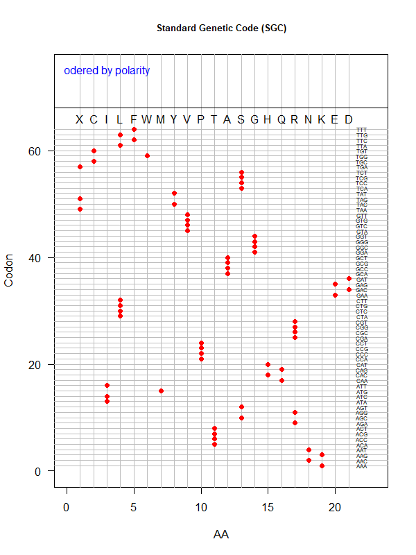
SGC: ordered by polarity
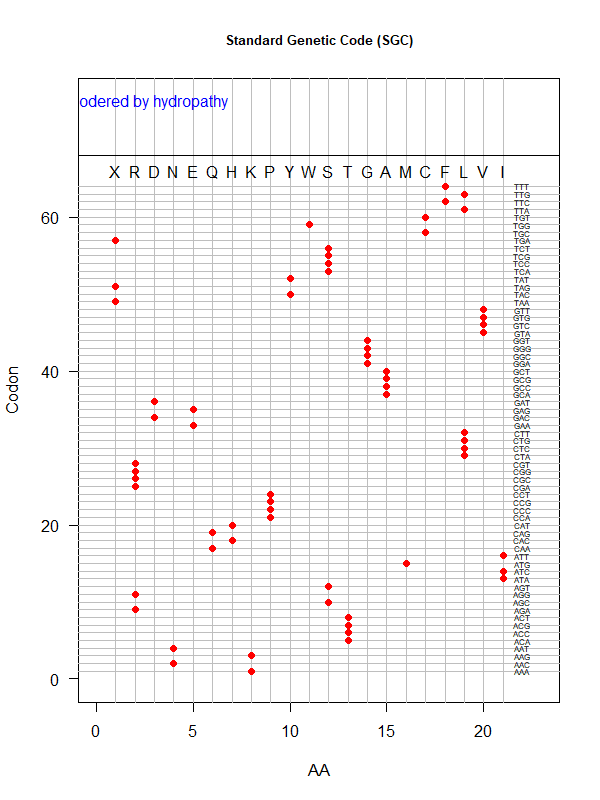
SGC: ordered by hydropathy
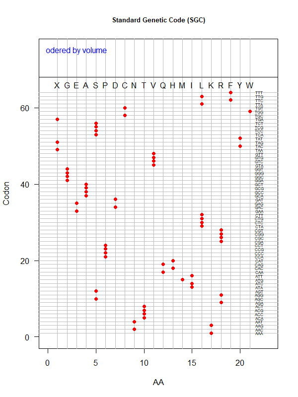
SGC: ordered by volume
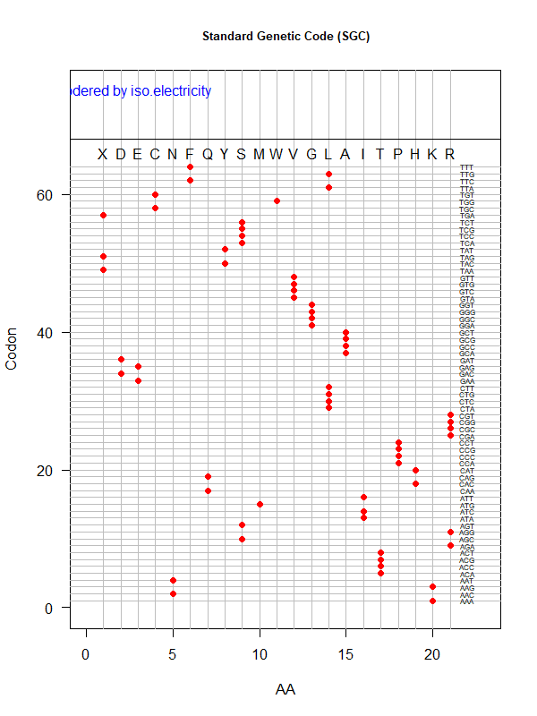
SGC: ordered by isoelectricity
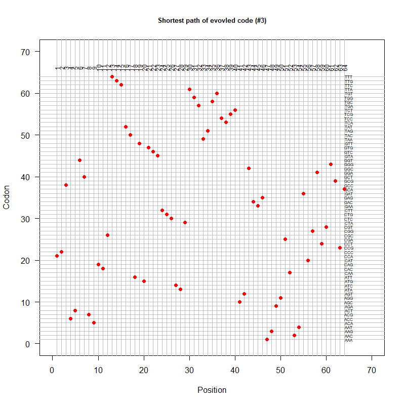
An evolved code (by Oliver)
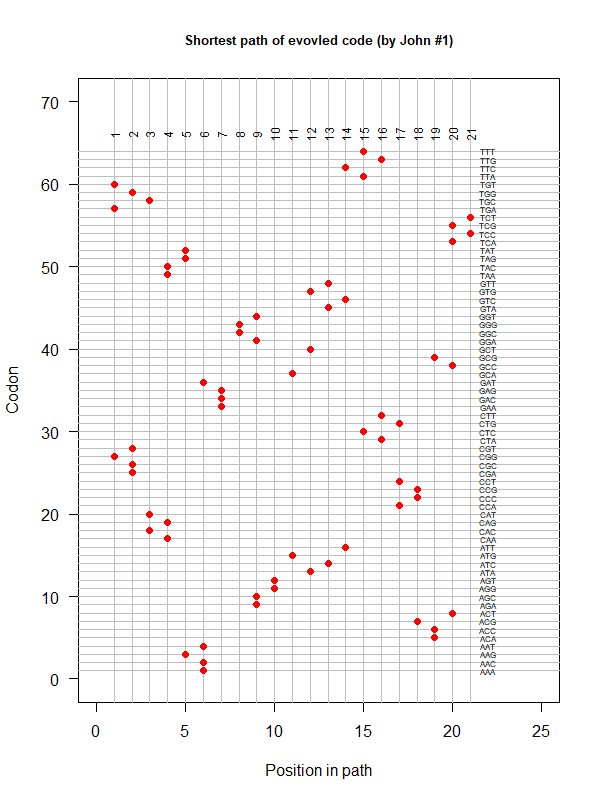
An evolved code (by John). Round-trip (last position connected with the first) AA assigned according to polarity gradient & with "TAA" as the 1st.
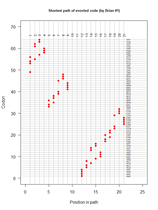
An evolved code (by Brian). One-way tour (last position NOT connected with the first). AA assigned according to polarity gradient & with "TAA" as the 1st.
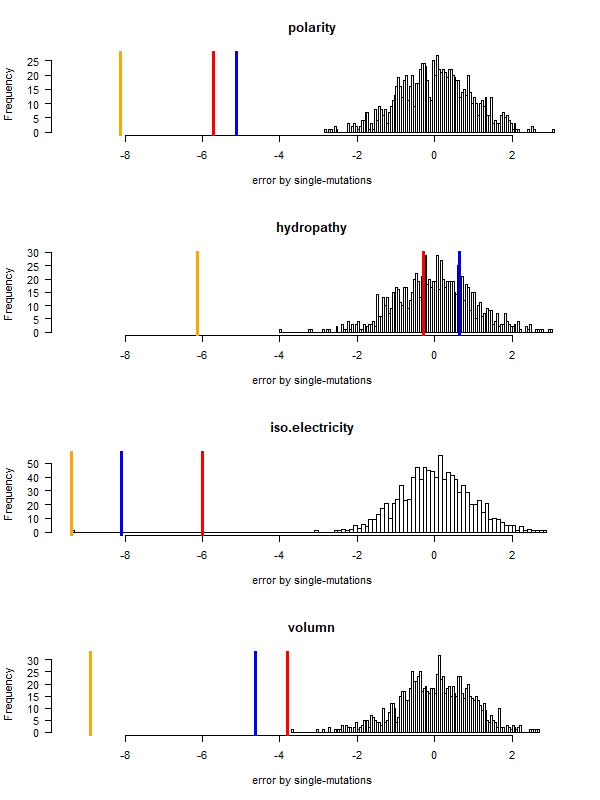
code robustness: SGC, John's simulated code , Brian's simulated code , histogram: 1000 random codes. X-axis: mean-squared error (standardized) caused by single-nt substitutions. Evolved codes perform better than SGC!
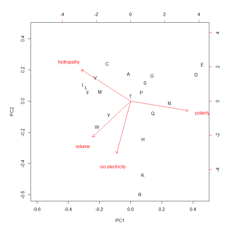
PC1 (mostly polarity and hydropathy, anti-correlated) & PC2 (the other two, positively correlated) of 4 AA metrics. PC1 and PC2 could be used for AA ranking as composite variables
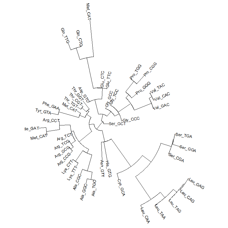
A tRNA gene tree from Aeropyrum pernix (an Archaea). Sequences from an rRNA database. Structual alignment available
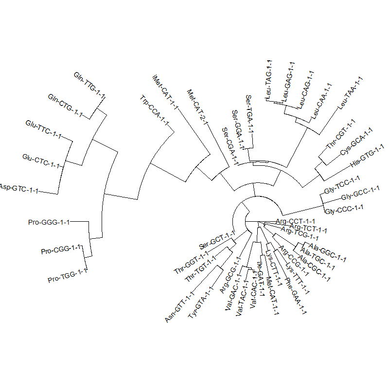
tRNA gene tree for Pyrococcus horikoshii (another Archaea). Sequences from UCSD tRNA database. (Not structurally aligned; only fasta seqs available)
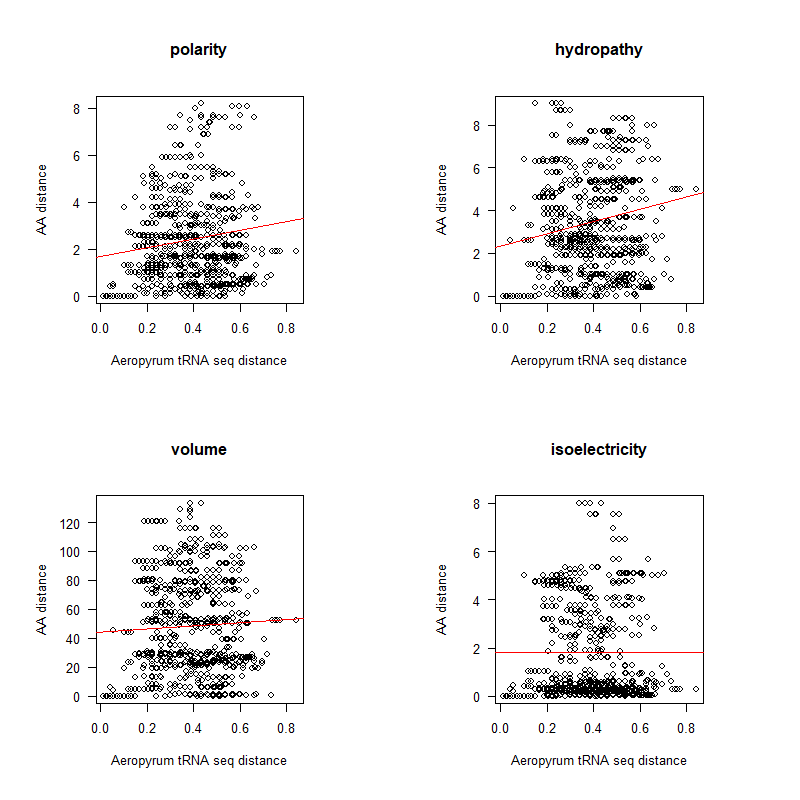
AA distance appears to be correlated with tRNA seq differences (especially at low distances)


- Participants: Oliver, John, Brian
- A representation mimicking TSP (see figure at right)
- Code to calculate total (mutational, ti/tv) path of SGC?
- Code to calculate energy of SGC?
- Randomize amino acid assignment and obtain distributions of path & energy
- Code to minimize total path length and energy?
- How to evolve a robust SGC? mutation bias + polarity/hydropathy + usage
Season I. Spring 2017 (Themes: Dueling Idiots/Digital Dice/Wright Fisher Process)
"Coalescence" (Backward simulation of Wright-Fisher process) (Due May 12, 2017)


We will conclude Spring 2017 season with the coalescence simulation (in summer, we will start experimenting with simulation of systems evolution)
Previously, we simulated Wright-Fisher process of genetic drift (constant pop size, no selection) starting from a founder population and end with the present population. This is not efficient because the program has to track each individual in each generation, although the majority of them do not contribute to the present population.
Coalescence simulation takes the opposite approach of starting from the present sample of k individuals and trace backward in time to their most recent common ancestor (MRCA). Due to the nature of Poisson process, the waiting time from one coalescence event (at time T) to the next one (at time T-1) is exponentially distributed with a mean of (k choose 2) generations. This process is iterated until the last coalescent event.
The classic text on coalescence is Richard Hudson's chapter, which includes (in Appendix) C codes for simulating tree and mutations. Hudson is also the author of ms, the widely used coalescence simulator.
Like the ms 10 1 -T command, your code should output a tree of 10 individuals. [A lot tougher than I thought; can't figure it out in R; so I did it in Perl]. Similarly, you could use R, where the ape package has a function called rcoal() that generate a random coalescence tree. Try this command: plot(rcoal(10)) (first load library by running library(ape)).
| Submitted Codes |
|---|
#!/usr/bin/env perl
# Basic coalescence
# First, simulate coalescent events with recursion
# Second, use Bio::Tree to export a newick tree
use strict;
use warnings;
use Data::Dumper;
use Algorithm::Numerical::Sample  qw /sample/;
use Math::Random qw(random_exponential);
use Bio::Tree::Tree;
use Bio::Tree::Node;

######################
# Initialize
######################
die "Usage: $0 <num-of-samples>\n" unless @ARGV == 1;
my $nsamp = shift @ARGV;
my @samples;
for (my $i=1; $i<=$nsamp; $i++) { push @samples, {id=>$i, parent=>undef, br=>0} }
my $ctr = $nsamp;
my $time = 0;
my @all_nodes;

################################################################################
# Simulate events with exponential time intervals between two successive events
#################################################################################
&coal(\@samples, \$ctr, \$time);
#print Dumper(\@all_nodes);
#########################################
# Reconstitute into tree using Bio::Tree
##########################################
my %seen_node;
my $max_id=0;
my @nodes;
foreach (@all_nodes) {
    $max_id = ($_->{parent} > $max_id) ? $_->{parent} : $max_id;
    if ($seen_node{$_->{id}}) { # child exist, previously as a parent, no branch length
        $seen_node{$_->{id}}->branch_length(sprintf "%.6f", $_->{br}); # add branch length
        if ($seen_node{$_->{parent}}) { # parent exist
            $seen_node{$_->{parent}}->add_Descendent($seen_node{$_->{id}});
        } else { # parent new
            my $pa = Bio::Tree::Node->new(-id=>$_->{parent});
            $pa->add_Descendent($seen_node{$_->{id}});
            $seen_node{$_->{parent}} = $pa;
        }
    } else { # child new
        my $new = Bio::Tree::Node->new(-id=>$_->{id}, -branch_length => sprintf "%.6f", $_->{br});
        $seen_node{$_->{id}} = $new;
        if ($seen_node{$_->{parent}}) { # parent exist
            $seen_node{$_->{parent}}->add_Descendent($new);
        } else { # parent new
            my $pa = Bio::Tree::Node->new(-id=>$_->{parent});
            $pa->add_Descendent($new);
            $seen_node{$_->{parent}} = $pa;
        }
    }
}

#my $root = $seen_node{$max_id};
my $tree=Bio::Tree::Tree->new(-id=>'coal-sim', -node=>$seen_node{$max_id}, -nodelete=>1);
print $tree->as_text("newick"), "\n";

exit;

sub coal {
    my $ref_nodes = shift;
    my $ref_ct = shift;
    my $ref_time = shift;
    my $ct = $$ref_ct;
    my @current_nodes = @$ref_nodes;
    my $k = scalar @current_nodes;
    my @new_nodes;
    return unless $k > 1;
    my @pair = sample(-set => $ref_nodes, -sample_size => 2);
#    print $ct, "\t", $$ref_time, "\t", $pair[0]->{id}, "\t", $pair[1]->{id}, "\n";
    $$ref_time += random_exponential(1, 2/$k/($k-1));
    my $new_nd = {id=>$ct+1, parent=>undef, br=>$$ref_time};
    map {$_->{parent} = $ct+1} @pair;
    map {$_->{br} = $$ref_time - $_->{br}} @pair;
    push @all_nodes, $_ for @pair;
    foreach (@current_nodes) {
        push @new_nodes, $_ unless $_->{id} == $pair[0]->{id} || $_->{id} == $pair[1]->{id};
    }
    push @new_nodes, $new_nd;
    $$ref_ct++;
    &coal(\@new_nodes, $ref_ct, $ref_time);
}
from Bio import Phylo
from io import StringIO
from random import sample
from scipy.misc import comb
from itertools import combinations
from numpy.random import exponential as exp

# Generate Random Tree with Nodes & Waiting Time
individuals = ["A", "B", "C", "D", "E", "F", "G", "H", "I", "J"]
node_dict = {}
reference = {}
wait_time_ref = {}
node = 0
while len(individuals) != 1:
    node_dict[node] = {"child_nodes": []}
    sample_events = tuple(sample(individuals, 2))
    reference[sample_events] = node
    wait_time = exp(1/comb(len(individuals), 2))
    wait_time_ref[node] = wait_time
    for sample_event in sample_events:
        if type(sample_event) == str:
            node_dict[node]["child_nodes"].append(sample_event)
        else:
            child_node = reference[sample_event]
            node_dict[node]["child_nodes"].append(child_node)
    individuals.remove(sample_events[0])
    individuals.remove(sample_events[1])
    individuals.append(sample_events)
    node += 1

# Calculate Tree Branch Lengths
tree_dict = {}
cumulative_br_length = 0
cumulative_br_len_dict = {}
for i in range(len(node_dict)):
    tree_dict[i] = {}
    cumulative_br_length += wait_time_ref[i]
    cumulative_br_len_dict[i] = cumulative_br_length
    for node in node_dict[i]['child_nodes']:
        if type(node) == str:
            tree_dict[i][node] = cumulative_br_length
        else:
            tree_dict[i][node] = cumulative_br_len_dict[i] - cumulative_br_len_dict[node]

# Parse the Tree into a String
for i in range(len(tree_dict)):
    for node in tree_dict[i].keys():
        if type(node) != str:
            temp = str(tree_dict[node])
            tree_dict[i][temp] = tree_dict[i].pop(node)
tree_str = str(tree_dict[i]).replace('\'', '').replace('\"', '').replace('\\', '').replace('{', '(').replace('}', ')').replace(' ', '')
tree_str += ";"

# Visualize Tree
handle = StringIO(tree_str)
tree = Phylo.read(handle, 'newick')
tree.ladderize()   # Flip branches so deeper clades are displayed at top
Phylo.draw(tree)
|
April 17, 2017 "Mutation Meltdown" (Due May 5, 2017)

Our last exploration showed that population will reach a steady-state level of DNA sequence polymorphism under the opposing forces of genetic drift and mutations. The steady-state level is expected to be ~ N * mu: the larger the population size and the higher the mutation rate, the higher per-site DNA polymorphism. (Also note that, given a long enough sequence and a low enough mutation rate, we don't expect to see two or more mutations hitting a single position. Each mutation is essentially a new one and only two-state SNPs are expected in a sample of DNA sequences).
However, the steady-state expectation is based on the assumption that all mutations are neutral (i.e., no beneficial or harmful fitness effects). In reality, mutations are predominantly either neutral or harmful and few are beneficial. Natural selection (negative or positive, except those on the immune-defense loci) tends to drive down genetic variation.
Sex to the rescue. Without sex or recombination, the fate of genetic variations across a genome are bundled together, rising or sinking in unison with the fate of a single beneficial or harmful mutation. With recombination, genetic variations at different loci become less tightly linked and are more likely maintained, speeding up adaptation.
This week, we will use simulation to recreate the so-called "Muller's Ratchet", which predicts that asexual populations are evolutionary dead ends. It shows that the combined effect of deleterious mutation and genetic drift will lead to population extinction due to steady accumulation of deleterious mutations, a phenomenon called "mutation meltdown".
The simulation protocol would be similar to that of the last problem involving only mutation and drift, but I suggest you rewrite from scratch to be more efficient by using a simpler data structure (no sequence or bases needed). The main difference is that, instead of calculating average pairwise sequence differences in each generation, you will track the frequency of mutation-free sequences (n0) and find the time until it goes to zero. That is when the Ratchet makes a "click". The next click is when the population losses the one-mutation sequences (n1), and so on. Each click drives the population fitness down by one mutation-level. [ Numerically, if each mutation causes a fitness loss of s ("selection coefficient"), the fitness of a sequence with k mutations is given by w = (1-s)k. Strictly speaking, the selection coefficient should be included to affect gamete size, but let's ignore that for now].
If there is recombination, the mutation-free sequences could be recovered (simulation next time?). Without recombination, the only direction for the population to evolve is a steady loss of best-fit individuals (by genetic drift).
Questions:
- Does the ratchet occur faster in small or large populations? Find by simulating N=100 and N=1000
- Does the ratchet occur faster for a short or long genome? Find by simulating L=1e3 and L=1e4
- Which parts of the human genomes are asexual (therefore subject to Muller's Ratchet and becoming increasingly small)?
| Submitted Codes |
|---|
import numpy as np
import matplotlib.pyplot as plt
from numpy.random import poisson
from numpy.random import choice

def simulator(seq_length, pop, repro_rate, generations):
    mutation_rate = 0.00001
    lam = seq_length * mutation_rate
    individuals = np.array([1 for i in range(pop)])
    non_mutated_pop_rate = []
    for generation in range(generations):
        gametes = []
        for individual in individuals:
            off_sprs = poisson(lam, repro_rate)
            mutation_ix = np.array(np.where(off_sprs != 0))
            indiv_gametes = np.array([individual for j in range(repro_rate)])
            indiv_gametes[mutation_ix] = 0
            gametes += list(indiv_gametes)
        individuals = choice(gametes, size=pop)
        non_mutated_frequency = float(np.count_nonzero(individuals)) / pop
        non_mutated_pop_rate.append(non_mutated_frequency)
    return non_mutated_pop_rate

genome_length_1000 = 1000
genome_length_10000 = 10000
results_1000 = simulator(genome_length_1000, 1000, 100, 500)
results_10000 = simulator(genome_length_10000, 1000, 100, 500)

genome_length_1000 = 1000
genome_length_10000 = 10000
results2_1000 = simulator(genome_length_1000, 10000, 100, 500)
results2_10000 = simulator(genome_length_10000, 10000, 100, 500)

f, (ax1, ax2) = plt.subplots(1, 2, sharey=True)
line_1_1000 = ax1.plot(results_1000, "r")
line_1_10000 = ax1.plot(results_10000, "b")
line_2_1000 = ax2.plot(results2_1000, "r")
line_2_10000 = ax2.plot(results2_10000, "b")

ax1.set_title("Population = 1000")
ax2.set_title("Population = 10000")

plt.title("Mutation Meltdown")
plt.show()
add.mutation <- function(genome, genome.length, mutation.rate) {
  mu.exp <- genome.length * mutation.rate;
  mu.num <- rpois(1, lambda = mu.exp);
  return(genome+mu.num);
}

ratchet <- function(pop.size=100, gamete.size=100, mu=1e-4, genome.length=1e4) {
  out <- data.frame(generation=numeric(), n0=numeric(), n1=numeric(), pop=numeric(), length=numeric());
  pop <- rep(0, pop.size) # initial all mutation-free
  g <- 1; # generation
  freq0 <- 1; # freq of zero-class
  while(freq0 > 0) {
    cat("at generation", g, "\n");
    freq0 <- length(which(pop == 0));
    out <- rbind(out, data.frame(generation=g, n0=freq0/pop.size, pop=pop.size, length=genome.length));
    gametes <- sapply(1:gamete.size, function(x) {lapply(pop, function(x) add.mutation(x, genome.length, mu))});
    pop <- sample(gametes, pop.size);
    g <- g+1;
  }
  return(out);
}

out.long.genome.df <- ratchet(genome.length=1e4);
out.short.genome.df <- ratchet(genome.length=1e3); |
March 31, 2017 "Drift-Mutation Balance" (4/14/2017)

We will explore genetic drift of a DNA fragment with mutation under Wright-Fisher model. From last week's exercise, we conclude that a population will sooner or later lose genetic diversity (becoming fixed after ~2N generations), if no new alleles are generated (by e.g., mutation or migration).
Mutation, in contrast, increases genetic diversity over time. Under neutrality (no natural selection against or for any mutation, e.g., on an intron sequence), the population will reach an equilibrium point when the loss of genetic diversity by drift is cancelled out by increase of genetic diversity by mutation.
You job is to find this equilibrium point by simulation, given a population size (N) and a mutation rate (mu). The expected answer is pi=2N*mu, where pi is a measure of genetic diversity using DNA sequences, which is the average pairwise sequence differences within a population.
Note: the following algorithm seems to be too complex to build at once. Also, too slow to run in R. Nonetheless, please try to write two R functions: (1)mutate.seq(seq, mut), with "seq" as a vector of bases and "mut" is the mutation rate, and (2) avg.seq.diff(pop), with "pop" as a list of DNA sequences
A suggested algorithm is:
- Start with a homogeneous population with N=100 identical DNA sequences (e.g., with a length of L=1e4 bases, or about 5 genes) [R hint:
dna <- sample(c("a", "t", "c", "g"), size=1e5, replace=T, prob = rep(0.25,4))] - Write a mutation function, which will mutate the DNA based on Poisson process (since mutation is a rare event). For example, if mu=1e-4 per generation per base per individual (too high for real, but faster for results to converge), then each generation the expected number of mutations would be L * mu = 1 per individual per generation for our DNA segment. You would then simulate the random number of mutations by using the R function
num.mutations <- rpois(1,lambda=1). - Apply the mutation function for each individual DNA copy (a total of N=100) during gamete production (100 gametes for each individual) at each generation (for a total of G=1000 generations).
- Write another function to calculate, for each generation, instead of counting allele frequencies (as last week's problem), to calculate & output average pairwise differences among the 100 individuals.
- Finally, you would graph pi over generation.
| Submitted Codes |
|---|
import numpy as np
import matplotlib.pyplot as plt
from itertools import combinations
from random import sample
from numpy.random import choice
from numpy.random import poisson

# global variables
nuc = np.array(["A", "T", "C", "G"])
expected_mutation_rate = 0.00001 # there are 2 sequences per individual
seq_length = 10000
individual_pop = 100
gamete_rate = 100
generation = 1000

def simulator(population, repro_rate, generation):
    observed_mutation_collection = []

    # Original Individuals
    original = choice(nuc, seq_length, 0.25)
    individual_total = [original for i in range(population)]

    for i in range(generation): # iterate over 1000 generations
        # Produce Gametes
        gametes = []
        for individual in individual_total:
            gametes += [individual for i in range(repro_rate)]
        gametes = np.array(gametes)
        gametes_pop = gametes.shape[0] # number of gametes: 100 * 100

        # Mutation
        mutation_number_arr = poisson(lam=seq_length * expected_mutation_rate, size=gametes_pop) # derive number of mutations per individual
        mutation_index_arr = [sample(range(seq_length), mutations) for mutations in mutation_number_arr] # get the index of mutation
        # Mutation: Replace with Mututated Base Pairs
        for i in range(gametes_pop): # iterate over all gametes
            for ix in mutation_index_arr[i]: # iterate over mutated base pair for each gamete
                gametes[i, ix] = choice(nuc[nuc != gametes[i, ix]], 1)[0] # locate mutation and alter the nuc with mutated one

        # Next generation of individuals
        individual_total = gametes[choice(range(10000), 100, replace=False)]

        # Calculate observed mutation rate
        num_combinations = 0
        total_diff_bases = 0
        for pair in combinations(range(len(individual_total)), 2): # aggregate mutations for all possible pairs of individuals
            total_diff_bases += len(np.where((individual_total[pair[0]] == individual_total[pair[1]]) == False)[0])
            num_combinations += 1
        observed_mutation_rate = float(total_diff_bases) / float(num_combinations) / seq_length
        observed_mutation_collection.append(observed_mutation_rate)

    return(observed_mutation_collection)

# Simulation
result = simulator(100, 100, 1000)

# Visualize results
plt.plot(result, 'b')
plt.xlabel("Generation")
plt.ylabel("Mutation Rate")
plt.title("Drift-Mutation Balance")
plt.show()
library(Biostrings) # a more compressed way to store and manipulate sequences
bases <- DNA_ALPHABET[1:4];
dna <- sample(bases, size = 1e5, replace = T);
library(ape) # to use the DNAbin methods
# function to mutate (Poisson process)
mutate.seq <- function(seq, mutation.rate) {
  mu.exp <- length(seq) * mutation.rate;
  mu.num <- rpois(1, lambda = mu.exp);
  if (mu.num > 0) {
    pos <- sample(1:length(seq), size = mu.num);
    for (j in 1:length(pos)) {
      current.base <- seq[pos[j]];
      mutated.base <-sample(bases[bases !=current.base)], size = 1);
      seq[pos[j]] <- mutated.base;
    }
  }
  return(seq)
}

# main routine
drift.mutation <- function(pop.size=100, generation.time=500, gamete.size=10, mu=1e-5) {
  out <- data.frame(generation=numeric(), pi=numeric()); # for storing outputs
  pop <- lapply(1:pop.size, function(x) dna)  # create the initial population
  for(i in 1:generation.time) { # for each generation
    cat("at generation", i, "\n"); # print progress
    gametes <- sapply(1:gamete.size, function(x) {lapply(pop, function(x) mutate.seq(x, mu))});
    pop <- sample(gametes, pop.size);
    pop.bin <- as.DNAbin(pop); # change into DNAbin class to advantage of its dist.dna() function
    out <- rbind(out, data.frame(generation=i, pi=mean(dist.dna(pop.bin))));
  }
  out;
}
out.df <- drift.mutation(); # run function and save results into a data frame
|
March 18, 2017 "Genetic Drift" (Due 3/31/2017)


This is our first biological simulation. Mandatory assignment for all lab members (from interns to doctoral students). An expected result is shown in the graph.
Task: Simulate the Wright-Fisher model of genetic drift as follows:
- Begin with an allele frequency p=0.5, and a pop of N=100 haploid individuals [Hint:
pop <- c(rep("A", 50), rep("a", 50))] - Each individual produces 100 gametes, giving a total of 10,000 gametes [Hint: use a for loop with rep() function]
- Sample from the gamete pool another 100 to give rise to a new generation of individuals [Hint: use sample() function]
- Calculate allele frequency [Hint: use table() function]
- Repeat the above in succession for a total generation of g=1000 generations [Hint: create a function with three arguments, e.g., wright.fisher(pop.size, gamete.size, generation.time)]
- Plot allele frequency changes over generation time
- Be prepared to answer these questions:
- Why allele frequency fluctuate even without natural selection?
- What's the final fate of population, one allele left, or two alleles coexist indefinitely?
- Which population can maintain genetic polymorphism (with two alleles) longer?
- Which population gets fixed (only one allele remains) quicker?
| Submitted Codes |
|---|
#Simple sampling, haploid, as a function
wright_fisher <- function(pop_size, gam_size, alle_frq, n_gen) {
  pop <- c(rep("A", pop_size*frq), rep("a", pop_size*frq))
  prob <- numeric(n_gen)
  for(time in 1:n_gen){
    gamt <- rep(pop, gam_size)
    pop <- sample(gamt, pop_size)
    prob[time] <- table(pop)[1]/pop_size
  }
  wf_df <- data.frame(generation=1:n_gen, probability=prob)
  plot(drift_df, type= 'l', main = "Wright-Fisher Process (Genetic Drift)", xlab = "generation", ylab = "allele frequency")
}

wright_fisher(1000, 100, 0.5, 1000)

#Version 2. Using binomial distribution with replicates, diploid

pop_size <- c(50, 100, 1000, 5000)
alle_frq <- c(0.01, 0.1, 0.5, 0.8)
n_gen <- 100
n_reps <- 50
genetic_drift <- data.frame()

for(N in pop_size){
  for(p in alle_frq){
    p0 <- p
    for(j in 1:n_gen){
      X <- rbinom(n_reps, 2*N, p)
      p <- X/(2*N)
      rows <- data.frame(replicate= 1:n_reps, pop=rep(N, n_reps), gen=rep(j, n_reps), frq=rep(p0, n_reps), prob=p )
      genetic_drift <- rbind(genetic_drift, rows)
    }
  }
}

library(ggplot2)
ggplot(genetic_drift, aes(x=gen, y=prob, group=replicate)) + geom_path(alpha= .5) + facet_grid(pop ~ frq) + guides(colour=FALSE)

# 3rd version: trace ancestry (instead of allele frequency)
#Python
import numpy as np
import sys
from random import sample
import matplotlib.pyplot as plt

def simulator(gametes_rate, next_individuals, generations):
    individuals = [1 for i in range(50)] + [0 for j in range(50)]
    frequency = []
    for generation in range(generations):
        gametes = []
        for individual in individuals:
            gametes += [individual for i in range(gametes_rate)]
        individuals = sample(gametes, next_individuals)
        frequency.append(np.count_nonzero(individuals) / len(individuals))
    return(frequency)

N_100 = simulator(100, 100, 1000)
N_1000 = simulator(100, 1000, 1000)

# Create plots with pre-defined labels.
# Alternatively,pass labels explicitly when calling `legend`.
fig, ax = plt.subplots()
ax.plot(N_100, 'r', label='N=100')
ax.plot(N_1000, 'b', label='N=1000')

# Add x, y labels and title
plt.ylim(-0.1, 1.1)
plt.xlabel("Generation")
plt.ylabel("Frequency")
plt.title("Wright-Fisher Model")

# Now add the legend with some customizations.
legend = ax.legend(loc='upper right', shadow=True)

# The frame is matplotlib.patches.Rectangle instance surrounding the legend.
frame = legend.get_frame()
frame.set_facecolor('0.90')

# Set the fontsize
for label in legend.get_texts():
    label.set_fontsize('large')

for label in legend.get_lines():
    label.set_linewidth(1.5)  # the legend line width
plt.show()
#Scala
import scala.util.Random
import scala.collection.mutable.ListBuffer

val gamete_rate = 100
val offspr_rate = 100
val generations = 1000

var frequency: List[Double] = List()

var individuals = List.fill(50)(0) ++ List.fill(50)(1)

for(generation <- 1 to generations){
  var gametes = individuals.map(x => List.fill(gamete_rate)(x)).flatten
  individuals = Random.shuffle(gametes).take(offspr_rate)
  frequency = frequency :+ individuals.count(_ == 1).toDouble / offspr_rate
}

print(frequency)
#Spark
val gamete_rate = 100
val offspr_rate = 100
val generations = 300

var frequency: List[Double] = List()
var individuals = sc.parallelize(List.fill(50)("0") ++ List.fill(50)("1"))

for(generation <- 1 to generations){
  val gametes = individuals.flatMap(x => (x * gamete_rate).split("").tail)
  individuals = sc.parallelize(gametes.takeSample(false, offspr_rate))
  val count = individuals.countByValue
  frequency = frequency :+ count("1").toDouble / offspr_rate
}

print(frequency)
Wright<-function(pop.size,gam.size,generation) {
 if( pop.size%%2==0) {

  pop<-c(rep("A",pop.size*.5),rep("a",pop.size))
  frequency<-.5
  time<-0
  geneticDrift<-data.frame(frequency,time)
  for (i in 1:generation) {
    largePop<-rep(pop,gam.size)
    samplePop<-sample(largePop,100)
    cases<-table(samplePop)
    if (cases[1]<100 && cases[2]<100 )
        {propA<-(cases[1]/100)
        geneticDrift<-rbind(geneticDrift,c(propA,i))
        pop<-c(rep("A",cases[2]),rep("a",cases[1]))
  }
}
  plot(geneticDrift$frequency~geneticDrift$time,type="b", main="Genetic Drift N=1000", xlab="time",ylab="Proportion Pop A",col="red", pch=18 )
}
 if(pop.size%%2==1 ) {
   print("Initial Population should be even. Try again")
 }
}
Wright(1000,100,1000)
Genetic_code = function(t,R){
  N<- 100
  p<- 0.5
  frequency<-as.numeric();
  for (i in 1:t){
    A1=rbiom(1,2*N,p)
    p=A1/(N*2);
    frequency[length(frequency)+1]<-p;
  }
  plot(frequency, type="1",ylim=c(0,1),col=3,xlab="t",ylab=expression(p(A[1])))

  }
p=0.5
N=100
g=0
pop <- c(rep("A", 50), rep("a", 50)) #create a population of 2 alleles
data<-data.frame(g,p) #a set of variables of the same # of rows
for (i in 1:1000) { #generation
  gam_pl <-rep(pop, 100) #gamete pool
  gam_sam <-sample(gam_pl, 100)  #sample from gamete pool
  tab_all<-table(gam_sam) #table ps sample
  all_freq<-tab_all[1]/100 #get allele frequency
  data<-rbind(data, c(i,all_freq))
  pop<-c(rep("A",tab_all[1]))
}
plot(data$g,data$p)
pop <- c(rep("A", 50), rep("a", 50))
wright_fisher <- function(N,gen_time,gam) {
  N=N
  gen_time = gen_time
  x = numeric(gen_time)
  x[1] = gam
  for (i in 2:1000) {
  k=(x[i-1])/N
  n=seq(0,N,1)
  prob=dbinom(n,N,k)
  x[i]=sample(0:N, 1, prob=prob)

}

plot(x[1:gen_time], type="l", pch=10)

}
pool <- rep(pop, times = 100)
s_pool <- sample(pool, size = 100, replace = F)
table(s_pool)
wright_fisher2 <- function(pop_size,al_freq,gen_time) {
  pop <- c(rep("A", pop_size/2), rep("a", pop_size/2))
  pool <-rep(pop, times=100)
  s_pool <- sample(pool, size = 100, replace = T)
  for(i in 1:gen_time)
    s_pool <- sample(sample(pool, size = pop_size, replace = F))
  a.f <- table(s_pool)[1]/100
  return(a.f)
  }
N=100
p=0.5
g=1000
sim=100
Genetic_drift=array(0, dim=c(g,sim))
Genetic_drift[1,]=rep(N*p,sim)
for(i in 1:sim) {
  for(j in 2:g){
    X[j,i]=rbinom(1,N,prob=X[j-1,i]/N)
  }
}
Genetic_drift=data.frame(X/N)
matplot(1:1000, (X/N), type="l",ylab="allele_frequency",xlab="generations")
# output frequency:
wright.fisher <- function(pop.size, generation.time=1000, gametes.per.ind=100) {
  out.df <- data.frame(gen=numeric(), freq=numeric(), pop.size=numeric());
  pop <- c(rep("A", pop.size/2), rep("a", pop.size/2)); # initial pop
  for(i in 1:generation.time) {
    gametes <- unlist(lapply(pop, function(x) rep(x, gametes.per.ind)));
    pop <- sample(gametes, pop.size); # sample gamete pool without replacement
    freq.a <- table(pop)[1]/pop.size; # frequency of "a"
    out.df <- rbind(out.df, c(gen=i, freq=freq.a, pop=pop.size, rep=rep));
  }
  out.list;
}

out.1e2<-wright.fisher(100)
out.1e3<-wright.fisher(1000)
# Make Figure 1 above
plot(out.1e2[,1], out.1e2[,2], type = "l", las=1, ylim=c(0,1), xlab="generation", ylab="allele frequency", main="Wright-Fisher Process (Genetic Drift)", col=3, lwd=2)
lines(out.1e3[,1], out.1e3[,2], type = "l", col=2, lwd=2)
legend(400, 0.2, c("N=100", "N=1,000"), lty=1, col=3:2, cex=0.75)
abline(h=0.5, col="gray", lty=2)

# Second function to track founders (not frequency)
wright.fisher.2 <- function(pop.size, generation.time=1000, gametes.per.ind=100) {
  pop <- 1:100 # label founders
  out.list <- list(pop);
  for(i in 1:generation.time) {
    gametes <- unlist(lapply(pop, function(x) rep(x, gametes.per.ind)));
    pop <- sample(gametes, pop.size); # sample gamete pool without replacement
    out.list[[i+1]] <- pop;
  }
  out.list;
}

out.1ist<-wright.fisher.2(100)
# plot loss of genetic diversity by tracking surviving founder lineages
plot(x=1:100, y=rep(1, 100), ylim=c(0,100), xlim=c(1,600), type="n", las=1, main="Drift: Suvival of founder lineages\n(N=100)", cex.main=0.75, xlab="generation", ylab="founders")
for (i in 1:600) { points(rep(i,100), 1:100, col=colors()[out.list[[i]]], cex=0.5) }
for (i in 1:600) {points(rep(i,100), out.list[[i]], cex=0.2, col="yellow") }
|
March 11, 2017 "Stoplights" (Due 3/18/2017)

- Source: Paul Nahin (2008). "Digital Dice", Problem 18.
- Challenge: How many red lights, on average, will you have to wait for on your journey from a city block m streets and n avenues away from Belfer [with coordinates (1,1)]? (assuming equal probability for red and green lights)
- Note that one has only wait for green light when walking along either the north side of 69 Street or east side of 1st Avenue. On all other intersections, one can walk non-stop without waiting for green light by crossing in the other direction if a red light is on.
- Formulate your solution with the following steps:
- Start from (m+1,n+1) corner and end at (1,1) corner
- The average number of red lights for m=n=0 is zero
- Find the average number of red lights for m=n=1 by simulating the walk 100 times
- Increment m & n by 1 (but keep m=n), until m=n=1000
- Plot average number of red lights by m (or n).
| Submitted Codes |
|---|
import numpy as np
import matplotlib.pyplot as plt
import pandas as pd
from pandas import DataFrame
from random import sample
from itertools import combinations, permutations
from numpy import count_nonzero, array

def red_light(av, st):
    traffic_light = ["red_st", "red_av"]
    total_cross = av + st - 1
    while av != 0 and st != 0:
        if sample(traffic_light, 1)[0] == "red_st":
            av -= 1
        else:
            st -= 1
    rest_cross = av if av != 0 else st
    return(count_nonzero([sample([0, 1], 1) for corss in range(rest_cross)]))

df = DataFrame(0, index=np.arange(10), columns=np.arange(10))

simulation = 1000
for av in df.index:
    for st in df.index:
        df.loc[av, st] = sum(array([[red_light(av, st)] for n in range(simulation)])) / simulation

plt.imshow(df, cmap='hot', interpolation='nearest')
plt.xticks(np.arange(1, 10))
plt.yticks(np.arange(1, 10))
plt.title("Average Numbers Waiting for Red Light")
plt.xlabel("Number of Av")
plt.ylabel("Number of St")
plt.show()

df

# Recursive Function for Each Trial

from sys import stdout
av = 30
st = 30
n_space = [0]
traffic_light = ["red_st", "red_av"]
def route(av, st):
    if not av == st == 0:
        if sample(traffic_light, 1)[0] == "red_st":
            if av == 0:
                stdout.write("w_")
                n_space[0] += 1
                route(av, st - 1)
            else:
                stdout.write("\n" + " " * n_space[0] + "|")
                route(av - 1, st)
        else:
            if st == 0:
                stdout.write("\n" + " " * n_space[0] + "w" + "\n" + " " * n_space[0] + "|")
                route(av - 1, st)
            else:
                stdout.write("_")
                n_space[0] += 1
                route(av, st - 1)
route(av, st)
#!/usr/bin/env perl
use strict;
use warnings;

# Use recursion
my ($distx, $disty) = @ARGV;
my $num_red = 0; # keep red-light counts
print "-" x $distx, "\n"; # print a starting line
&walk($distx, $disty, \$num_red); # pass reference not value
exit;

sub walk {
    my ($x, $y, $ref) = @_;
    my $ct = $$ref;
    my $prob_red;
    if ($x == 1 && $y == 1) { # Reached destination
	print "*\n";
	print "-" x $distx, "\n"; # print the ending line
	print "reached Belfer after waiting for ", $ct, " red lights\n";
    }

    if ($x == 1 && $y > 1) { # Reached right-side end
	$prob_red = rand();
	if ($prob_red < 0.5) { # red light, wait
	    $ct++;
	    print "w\n", " " x ($distx-1);
	} else {
	    print "|\n", " " x ($distx-1);
	}
	&walk($x, $y-1, \$ct);
    }

    if ($x > 1 && $y == 1) { # Reached bottom
	$prob_red = rand();
	if ($prob_red < 0.5) { # red light, wait
	    $ct++;
	    print "w";
	} else { print "-"}
	&walk($x-1, $y, \$ct);
    }

    if ($x > 1 && $y > 1) {
	my $prob_across = rand(); # prob of walking right with green light
	if ($prob_across >= 0.5) { # move one block right
	    print "-";
	    &walk($x-1, $y, \$ct);
	} else { # red light, move one block down
	    print "|\n", " " x ($distx-$x);
	    &walk($x, $y-1, \$ct);
	}
    }
}
# In[26]:
def walk (walker):
    import random

    def just_walk (x):                                  #[1]
        if random.choice(["red_m_direction", "green_m"])=="green_m": x["loca"]["m"] -=1
        else: x["loca"]["n"] -=1
        return x
    def may_have_to_wait (dist,waited):                 #[2]
        if random.choice(["green","red"])=="red": waited += 1
        else: dist -= 1
        return (dist,waited)

    while (0 not in walker["loca"].values()):         #start walking
        walker = just_walk(walker)
    while (walker["loca"]["m"] !=0):       # if n =0 and m != 0
        (walker["loca"]["m"], walker["waited"]) = may_have_to_wait(walker["loca"]["m"],walker["waited"])
    while (walker["loca"]["n"] !=0):       # if m =0 and n != 0
        (walker["loca"]["n"], walker["waited"]) = may_have_to_wait(walker["loca"]["n"],walker["waited"])

    return walker["waited"]

def given_distance(m,n,rep):
    waited = list()
    for x in range(rep):
        walker={"loca":{"m":m,"n":n}, "waited":0}     #walker variable
        waited.append(walk(walker))
    return sum(waited)/len(waited)
# main
result=list()
for d in range(1000):                                  # set walking distance here
        result.append(given_distance (d,d,100))      # set rep here
import matplotlib.pyplot as plt                     # ploting
plt.plot(result); plt.show()

#[1] no reason to wait for ANY red before one of the distances (m or n) is exhausted. Assuming when light is green for m, it must be red for n, vise versa.
#[2] when one of the directions (m or n = 0), waiting cannot be avoided, start counting.
|
March 3, 2017 "PiE" (Due 3/10/2017)
- Source: Paul Nahin (2008). "Dueling Idiots", Problem 5.
- Challenge: obtain numerical values of Pi and E by simulations
- Simulate pi by

- Randomly generate 10,000 pairs of uniformly distributed numbers from 0 and 1 (simulating throwing darts onto the unit square shown at right)
- Count the number of points enclosed within the quarter-circle
- Calculate the pi value from this proportion
- Simulate e by
- Generate N random numbers from 0 to 1
- Divide into N equal-width bins between 0 and 1
- Count the number of bins Z that receive none of the random numbers
- Obtain e ~ N/Z (based on binomial sampling formula)
- Simulate N=1e2, 1e3, and 1e4
| Submitted Codes |
|---|
# simulate pi:
darts <- sapply(1:1000, function(x) { coords<- runif(2); return(ifelse(coords[1]^2+coords[2]^2 <= 1, 1,0)) })
pi <- 4*mean(darts)

# simulate e
N <- 1e3;
n <- runif(N);
cts <- numeric();
for(i in 1:(N-1)) {
  left <- i/N;
  right <- (i+1)/N;
  cts[i] <- length(which(n>=left & n < right))
}
e <- N/length(which(cts==0))
#Simulate pi
random <- 0; square <- 0;
for (i in 1:1000){
  random[[i]]<- runif(1,0,1)
square[[i]]<- sqrt(1-(random[i])^2)
}
plot(random, square)
areaofqc <- (pi/4)
ranleqc <- length(which(random <=areaofqc))
squleqc <- length(which(square<=areaofqc))

#Simulate e
e <- 0;
for(N in 1:1000) {
  numbers<-runif(N)
bin.size<-1/N
  non.empty<-as.integer(numbers/bin.size)
  z.empt<- N - length(table(non.empty))
  e<-c(e, N/z.empt)
  }
plot(e)
#When you throw a dart at the a unit square dartboard the Probability of hitting the portion of the circle radius with center=(0,0) inside the unit square is  pi/4.  We can say that hitting the 1/4 circle within the unit square with a dart is a bernoulli random variable where p=pi/4. Further, we can say E(bernoulli=hit)=pi/4.
# Imagine you are scoring the game of darts as follows- 1 point if you throw in the 1/4 circle and 0 points if you miss this space.
# If you throw 10000 darts you just did 10000 iid bernoulli trials. By the law of large numbers if we count the number of hits to the 1/4 circle of radius 1 and divide by number of darts thrown we will get something pretty close to E(beroulli) . Multiply that number by 4 and you have an estimate of Pi.

## Generate 10,000 pairs of points in the unit square with uniform distribution

x<-c(runif(1000000, min = 0, max = 1))
y<-c(runif(1000000, min = 0, max = 1))
point<-data.frame(x,y)

plot(point$x,point$y)
point.sub<-subset(point,y<=sqrt(1-x^2))

plot(point.sub$x,point.sub$y)

z<-4*nrow(point.sub)/1000000
z
error<-pi-z
error

## simulating exp
#It's a well that a binomial with large n and tiny p is a good estimate of the poisson random For this estimate lambda=np.  In this case n=10,000 and p=the probability of falling into a particular unit=1/10000.......
 simexp<-function (n) {
a<-c(runif(n,min=0,max=1))
b<-c()

for (i in 1:n) {
  c<-subset(a,(i-1)/n<a & a<=i/n)
  d<-length(c)
  b<-append(b,d)
}
bzero<-subset(b,b==0)
length(bzero)
print(n/length(bzero))
}
simexp(1000)
simexp(10000)
simexp(100000)
#python code
# Simulate pi
simulation = 10000
distances = np.array([pow(uniform(0, 1), 2) + pow(uniform(0, 1), 2) for i in range(simulation)])
pi = count_nonzero(distances < 1) / simulation * 4
pi

# Simulate e
total = 10000
ranges = [[x/total, (x+1)/total] for x in range(total)]
sample_space = [uniform(0, 1) for x in range(total)]
index = []
for i in range(total):
    if any(ranges[i][0] <= point <= ranges[i][1] for point in sample_space):
        index.append(i)
e = total / (total - len(set(index)))
e
|
Feb 24, 2017 "Idiots" (Due 3/3/2017)

- Source: Paul Nahin (2000), "Dueling Idiots". Problem #2: "When Idiots Duel"
- Game: Idiots A and B decide to duel with a gun in the following way: They will insert a single bullet into the gun's cylinder. The cylinder has a total of 6 slots. Idiot A will spin the cylinder and shoot at B. If the gun doesn't fire, then A will give the gun to B, who will spin the cylinder and then shoot at A. This back-and-forth duel will continue until one fool shoots (and kills) the other.
- Questions: (1) what is the probability that A will win (and B dies); (2) What is the average number of trigger pulls before someone dies?
| Submitted Codes |
|---|
gun <-c(1,0,0,0,0,0)
gun2 <- c(1,0,0,0,0,0)
deadman <-0 ;idiot1win <-0; idiot2win <- 0; nooned <- 0; total <- 0
 while(deadman < 1000){
  idiot1shot <-sample(gun)
  if (length(which(idiot1shot[1] == 1))){
    deadman <- deadman + 1
    idiot1win <- idiot1win + 1
  }else{
      idiot2shot <-sample(gun2)
      if (length(which(idiot2shot[1] == 1))){
        deadman <- deadman +1
        idiot2win <- idiot2win +1
      } else {nooned <- nooned + 1}
  }
  total <- total + 1
  }


deadman
idiot1win
idiot2win
nooned
total

p <- idiot1win/1000
p*100
takes2kill <- deadman/total
takes2kill*100
idiot1shot
idiot2shot
rounds <- sapply(1:1000, function(x) {
  alive <- 1;
  round <- 0;
  while(alive == 1){
    spin <- sample(c(0,0,0,0,0,1));
    round <- round + 1;
    if(spin[1] == 1) { alive <- 0 }
  }
  return(round)
})
prob.a.live <- length(which(rounds %% 2 == 0))
barplot(table(rounds)/1000, xlab="num rounds", ylab="Prob", main = "Sudden Death with a 6-slot gun (sim=1000)", las=1)
|
Feb 17, 2017 "Birthday" (Due 2/24/2017)

- Problem: What is the probability NONE of the N people in a room sharing a birthday?
- Randomly select N individuals and record their B-days
- Count the B-days NOT shared by ANY two individuals
- Repeat (for each N) 1000 times, and obtain probability by averaging the previous counts (i.e., divided by 1000)
- Vary N from 10 to 100, increment by 10
- Plot probability of no-shared B-Day (Y-axis) versus N (x-axis), with either a stripchart or boxplot, or both
| Submitted Codes |
|---|
N <- 0
samples <- 0;
prob.nodub <-0;
for(j in 10:100){
  counting.no.dups <- 0;
  test <- for(i in 1:1000){
  bdays <- sample(seq(as.Date('1990/01/01'), as.Date('1990/12/31'), by="day"), N, replace=T)
  dups <- duplicated(bdays, incomparables = FALSE)
  ch <-length(which(dups == TRUE))
    if(ch==0){
      counting.no.dups <- counting.no.dups +1
    }
    fine <- (counting.no.dups/1000)
  }
  print(N)
  print(fine)
  N <- N + 1
  samples[[j]] <- N
  prob.nodub[[j]] <- fine
}
plot(samples,prob.nodub, main="Birthday Simulation", xlab = "Sample Size", ylab = "Probability of no Duplicates", las =1)
days <- 1:365;

find.overlap <- function(x) { return(length(which(table(x)>1))) }

output <- sapply(1:100, function(x) { # num of people in the room
  ct.no.overlap <- 0;
  for (k in 1:100) {
    bdays <- sample(days, x, replace = T);
    ct <- find.overlap(bdays);
    if (!ct) { ct.no.overlap <- ct.no.overlap + 1}
  }
  return(ct.no.overlap);
})

plot(1:100, output/100, xlab="Group size", ylab = "Prob (no shared b-day)", las=1, main="B-day (sim=100 times)", type="l")
abline(h=0.5, lwd=2, col=2, lty=2)
abline(v=seq(0, 100, 5), col="gray")
|
Feb 10, 2017 "Dating" (Valentine's Day Special; Due 2/17/2017)

- Source: Paul Nahin (2008), "Digital Dice". Problem #20: "An Optimal Stopping Problem"
- Problem: What is the optimal time point when one should stop dating more people and settle on a mate choice (and live with the decision)
- Your best strategy is to date an initial sample of N individuals, rejecting all, and marry the next one ranked higher than any of your N individuals. The question is what is the optimal number for N.
- The problem could be investigated by simulating a pool of 10 individuals, ranked from 1-10 (most desirable being 1) and then take a sample of N
- You may only date one individual at a time
- You cannot go back to reach previously rejected candidates
- Simulate N from 0 to 9 (zero means marrying the first date, a sample size of zero)
- For each N, obtain the probability of finding the perfect mate (i.e., ranked 1st) by running simulation 1000 times
- Plot barplot of probability versus sample size N.
- Expected answer: N=4
| Submitted Codes |
|---|
pick.candidate <- function(min, array) {
  for (i in 1:length(array)) {
    if (array[i] < min) {
      return(array[i])
    } else {next}
  }
  return(0) # No 1. has been sampled and rejected
}
candidates <- 1:10;
output <- sapply(0:9, function(x) {
  ct <- 0;
  for(k in 1:1000) {
    if (x==0) { # no sample, marry the 1st guy
      sampled <- sample(candidates, 1);
      if (sampled == 1) {ct <- ct+1}
    } else {
      sampled <- sample(candidates, x);
      not.sampled <- candidates[-sampled];
      not.sampled <- sample(not.sampled);
      if (pick.candidate(min =  min(sampled), array = not.sampled) == 1) {ct <- ct+1}
    }
  }
  return(ct);
})
barplot(output/1e3, names.arg = 0:9, xlab = "number of sampled dates", las=1, main = "Optimal stopping for dating (N=10 candidates)", ylab = "Prob(marrying No.1)")
|
Feb 3, 2017 "US Presidents" (Due 2/10/2017)

- Download : 1st column is the order, 2nd column is the name, the 3rd column is the year of inauguration; tab-separated
- Your job is to create an R, Perl, or Python script called “us-presidents”, which will
- Read the table
- Store the original/correct order
- Shuffle/permute the rows and record the new order
- Count the number of matching orders
- Repeat Steps 3-4 for a 1000 times
- Plot histogram or barplot (better) to show distribution of matching counts
- Hint: For R, use the sample() function. For Perl, use the rand() function.
| Submitted Codes |
|---|
pres.list <- lapply(1:1000, function(x) pres[sample(nrow(pres)),])
cts <- sapply(pres.list, function(x) {
  ct.match <- 0;
  for (i in 1:45){
    if (pres$order[i] == x[i,1]){
      #cat(as.character(x[i,2]), x[i,1], "\n")  #as.character to avoid the factor info
      ct.match <- ct.match + 1;
      #cat(ct.match)
    }
  }
  ct.match #return
})
barplot(table(cts),xlab = "Number of matches per shuffle", border = "hotpink", col = "pink", ylab = paste("Frequency total of:",length(pres.list)), main = "US Presidents")
import pandas as pd
import numpy as np
from pandas import DataFrame
import matplotlib.pyplot as plt

df = pd.read_table("presidents.txt", names=["num", "name", "presidency"])

name_list = list(df.name)

# create a list to store matches after each shuffle
shuffle_record = []

# create a function in which the first argument is the original dataset; second argument is number of shuffles
def shuffler2(original, n):
    record = []
    for i in range(n):
        num = 0
        each_shuffle = {}
        temp = original.reindex(np.random.permutation(original.index)) # do shuffling for each
        compare = original.num == temp.num
        matched_df = original.ix[compare[compare == True].index]
        for i in matched_df.index:
            each_shuffle[i] = matched_df.name[i]
        shuffle_record.append(each_shuffle)
        try:
            num = compare.value_counts()[1]
        except:
            pass
        record.append(num)
    return(record)
result2 = shuffler2(df, 1000)

plt.hist(result2, color="yellow")
plt.title("Histgram for President Data")
plt.show()
p <- read.table("Presidents.txt", sep="\t", header=F)
colnames(p) <- c("order", "name", "inaug.year")
# Use "sapply" or "lapply" for loops: no need to pre-define a vector to store results
p.sim <- sapply(1:10000, function (x) {
  length(which(sample(p$order) == p$order))
  })
barplot(table(p.sim)/1e4, las=1)
p.exp <- rpois(1e4, 1) # draw 10000 Poisson random deviates
mp <- barplot(table(p.exp)/1e4, las=1, xlab = "Num of matching presidents") # mid-point on x-axis
lines(mp[1:7], table(p.sim)/1e4, type="b", col=2) # add a line (Poisson-expected) to the barplot (simulated)
legend("topright", c("Simulated", "Poisson expectation"), col=1:2, lty=1)
|