Monte Carlo Club: Difference between revisions
Jump to navigation
Jump to search
imported>Weigang |
imported>Weigang mNo edit summary |
||
| Line 12: | Line 12: | ||
# Plot barplot of probability versus sample size N. | # Plot barplot of probability versus sample size N. | ||
# Expected answer: N=4 | # Expected answer: N=4 | ||
{| class="wikitable sortable mw-collapsible" | |||
|- style="background-color:lightsteelblue;" | |||
! Submitted Codes | |||
|- style="background-color:powderblue;" | |||
| | |||
* By Weigang | |||
<syntaxhighlight lang="bash"> | |||
pick.candidate <- function(min, array) { | |||
for (i in 1:length(array)) { | |||
if (array[i] < min) { | |||
return(array[i]) | |||
} else {next} | |||
} | |||
return(0) # No 1. has been sampled and rejected | |||
} | |||
candidates <- 1:10; | |||
output <- sapply(0:9, function(x) { | |||
ct <- 0; | |||
for(k in 1:1000) { | |||
if (x==0) { # no sample, marry the 1st guy | |||
sampled <- sample(candidates, 1); | |||
if (sampled == 1) {ct <- ct+1} | |||
} else { | |||
sampled <- sample(candidates, x); | |||
not.sampled <- candidates[-sampled]; | |||
not.sampled <- sample(not.sampled); | |||
if (pick.candidate(min = min(sampled), array = not.sampled) == 1) {ct <- ct+1} | |||
} | |||
} | |||
return(ct); | |||
}) | |||
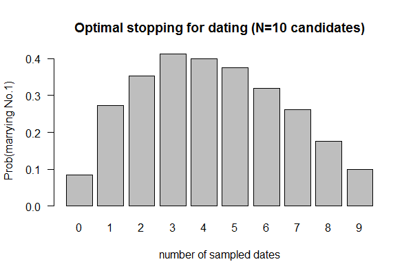
barplot(output/1e3, names.arg = 0:9, xlab = "number of sampled dates", las=1, main = "Optimal stopping for dating (N=10 candidates)", ylab = "Prob(marrying No.1)") | |||
</syntaxhighlight> | |||
|} | |||
==(Last week) Feb 3, 2017 "US Presidents" (Due 2/10/2017)== | ==(Last week) Feb 3, 2017 "US Presidents" (Due 2/10/2017)== | ||
[[File:Sim-presidents.png|thumbnail]] | [[File:Sim-presidents.png|thumbnail]] | ||
Revision as of 20:41, 18 February 2017
(This week) Feb 10, 2017 "Dating" (Valentine's Day Special; Due 2/17/2017)
- Source: Paul Nahin (2008), "Digital Dice". Problem #20: "An Optimal Stopping Problem"
- Problem: What is the optimal time point when one should stop dating more people and settle on a mate choice (and live with the decision)
- Your best strategy is to date an initial sample of N individuals, rejecting all, and marry the next one ranked higher than any of your N individuals. The question is what is the optimal number for N.
- The problem could be investigated by simulating a pool of 10 individuals, ranked from 1-10 (most desirable being 1) and then take a sample of N
- You may only date one individual at a time
- You cannot go back to reach previously rejected candidates
- Simulate N from 0 to 9 (zero means marrying the first date, a sample size of zero)
- For each N, obtain the probability of finding the perfect mate (i.e., ranked 1st) by running simulation 1000 times
- Plot barplot of probability versus sample size N.
- Expected answer: N=4
| Submitted Codes |
|---|
pick.candidate <- function(min, array) {
  for (i in 1:length(array)) {
    if (array[i] < min) {
      return(array[i])
    } else {next}
  }
  return(0) # No 1. has been sampled and rejected
}
candidates <- 1:10;
output <- sapply(0:9, function(x) {
  ct <- 0;
  for(k in 1:1000) {
    if (x==0) { # no sample, marry the 1st guy
      sampled <- sample(candidates, 1);
      if (sampled == 1) {ct <- ct+1}
    } else {
      sampled <- sample(candidates, x);
      not.sampled <- candidates[-sampled];
      not.sampled <- sample(not.sampled);
      if (pick.candidate(min =  min(sampled), array = not.sampled) == 1) {ct <- ct+1}
    }
  }
  return(ct);
})
barplot(output/1e3, names.arg = 0:9, xlab = "number of sampled dates", las=1, main = "Optimal stopping for dating (N=10 candidates)", ylab = "Prob(marrying No.1)")
|
(Last week) Feb 3, 2017 "US Presidents" (Due 2/10/2017)
- Download : 1st column is the order, 2nd column is the name, the 3rd column is the year of inauguration; tab-separated
- Your job is to create an R, Perl, or Python script called “us-presidents”, which will
- Read the table
- Store the original/correct order
- Shuffle/permute the rows and record the new order
- Count the number of matching orders
- Repeat Steps 3-4 for a 1000 times
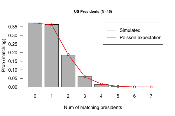
- Plot histogram or barplot (better) to show distribution of matching counts
- Hint: For R, use the sample() function. For Perl, use the rand() function.
| Submitted Codes |
|---|
pres.list <- lapply(1:1000, function(x) pres[sample(nrow(pres)),])
cts <- sapply(pres.list, function(x) {
  ct.match <- 0;
  for (i in 1:45){
    if (pres$order[i] == x[i,1]){
      #cat(as.character(x[i,2]), x[i,1], "\n")  #as.character to avoid the factor info
      ct.match <- ct.match + 1;
      #cat(ct.match)
    }
  }
  ct.match #return
})
barplot(table(cts),xlab = "Number of matches per shuffle", border = "hotpink", col = "pink", ylab = paste("Frequency total of:",length(pres.list)), main = "US Presidents")
import pandas as pd
import numpy as np
from pandas import DataFrame
import matplotlib.pyplot as plt

df = pd.read_table("presidents.txt", names=["num", "name", "presidency"])

name_list = list(df.name)

# create a list to store matches after each shuffle
shuffle_record = []

# create a function in which the first argument is the original dataset; second argument is number of shuffles
def shuffler2(original, n):
    record = []
    for i in range(n):
        num = 0
        each_shuffle = {}
        temp = original.reindex(np.random.permutation(original.index)) # do shuffling for each
        compare = original.num == temp.num
        matched_df = original.ix[compare[compare == True].index]
        for i in matched_df.index:
            each_shuffle[i] = matched_df.name[i]
        shuffle_record.append(each_shuffle)
        try:
            num = compare.value_counts()[1]
        except:
            pass
        record.append(num)
    return(record)
result2 = shuffler2(df, 1000)

plt.hist(result2, color="yellow")
plt.title("Histgram for President Data")
plt.show()
p <- read.table("Presidents.txt", sep="\t", header=F)
colnames(p) <- c("order", "name", "inaug.year")
# Use "sapply" or "lapply" for loops: no need to pre-define a vector to store results
p.sim <- sapply(1:10000, function (x) {
  length(which(sample(p$order) == p$order))
  })
barplot(table(p.sim)/1e4, las=1)
p.exp <- rpois(1e4, 1) # draw 10000 Poisson random deviates
mp <- barplot(table(p.exp)/1e4, las=1, xlab = "Num of matching presidents") # mid-point on x-axis
lines(mp[1:7], table(p.sim)/1e4, type="b", col=2) # add a line (Poisson-expected) to the barplot (simulated)
legend("topright", c("Simulated", "Poisson expectation"), col=1:2, lty=1)
|
(Future weeks) Feb 17, 2017 "Birthday" (Due 2/24/2017)
- Randomly select N individuals and record their B-days
- Count the B-days NOT shared by ANY two individuals
- Repeat (for each N) 1000 times, and obtain probability by averaging the previous counts divided by 1000
- Vary N from 10 to 100, increment by 10
- Plot probability of no-shared B-Day (Y-axis) versus N (x-axis), with either a stripchart or boxplot, or both

