Molecular Evolution (BIOL 375.00/790.64/793.03, Fall 2019)
Instructor: Dr Weigang Qiu, Professor, Department of Biological Sciences
Room: 926 HN (Seminar Room, North Building)
Hours: Mon. & Thur 4:10-5:25 pm
Office Hours: Belfer Research Building (Google Map) BB-402; Fridays 3-5pm or by appointment
Course Website: http://diverge.hunter.cuny.edu/labwiki/Biol375_2019
christopher.panlasigui47@myhunter.cuny.edu
Course Description
Molecular evolution is the study of the change of DNA and protein sequences through time. Theories and techniques of molecular evolution are widely used in species classification, biodiversity, comparative genomics, and molecular epidemiology. Contents of the course include:
- Population genetics, which is a theoretical framework for understanding mechanisms of sequence evolution through mutation, recombination, gene duplication, genetic drift, and natural selection.
- Molecular systematics, which introduces statistical models of sequence evolution and methods for reconstructing species phylogeny.
- Bioinformatics, which provides hands-on training on data acquisition and the use of software tools for phylogenetic analyses.
This 3-credit course is designed for upper-level biology-major undergraduates. Hunter pre-requisites are BIOL203, and MATH150 or STAT113.
Textbooks
- (Required) Graur, 2016, Molecular and Genome Evolution, First Edition, Sinauer Associates, Inc. ISBN: 978-1-60535-469-9. Publisher's Website (Student discount: a 15% discount and receive free UPS standard shipping)
http://www.sinauer.com/molecular-and-genome-evolution.html)
- (Recommended) Baum & Smith, 2013. Tree Thinking: an Introduction to Phylogenetic Biology, Roberts & Company Publishers, Inc.
Learning Goals
- Be able to describe evolutionary relationships using phylogenetic trees
- Be able to use web-based as well as stand-alone software to infer phylogenetic trees
- Understand mechanisms of DNA sequence evolution
- Understand algorithms for building phylogenetic trees
Links for phylogenetic tools
Exams & Grading
- Bonus for full attendance & active participation in classroom discussions.
- Assignments. All assignments should be handed in as hard copies only. Email submission will not be accepted. Late submissions will receive 10% deduction (of the total grade) per day.
- Three Mid-term Exams (30 pts each)
- Comprehensive Final Exam (50 pts)
Academic Honesty
While students may work in groups and help each other for assignments, duplicated answers in assignments will be flagged and investigated as possible acts of academic dishonesty. To avoid being investigated as such, do NOT copy anyone else's work, or let others copy your work. At the least, rephrase using your own words. Note that the same rule applies regarding the use of textbook and online resources: copied sentences are not acceptable and will be considered plagiarism.
Hunter College regards acts of academic dishonesty (e.g., plagiarism, cheating on examinations, obtaining unfair advantage, and falsification of records and official documents) as serious offenses against the values of intellectual honesty. The College is committed to enforcing the CUNY Policy on Academic Integrity and will pursue cases of academic dishonesty according to the Hunter College Academic Integrity Procedures.
Course Schedule
Part 1. Tree Thinking
- 8/29 (TH). Overview & Introduction. Textbook Chapter: "Introduction" (pages 1-3)
| Assignment 1 (10 pts; Due next class 9/5)
|
- (10 pts) Pre-test: Full credits will be given as long as each question is answered with some reasoning. In other words, it will NOT be graded on being right or wrong. It's an assessment tool, to be compared with later test outcomes to show teaching/learning results.
|
- 9/5 (TH). Introduction (Continued)
- R terminologies
- Object: variable that contains data (e.g., "iris")
- Object class: type of data (e.g., "data.frame", which is a table)
- Function: e.g., data(iris), which loads the data set called "iris"
- Function arguments: input and options (e.g., "iris" above)
- Tutorial: R & R-Studio (Bring your own computer)
- Lecture slides:
| Assignment 2 (5 pts; Due: next session)
|
R exercises
- Install R & R-studio (see "Links for phylogenetic tools" above)
- Open R-studio and install the "ape" package using the "Packages"->"Install" menu, located within the lower right window
- Type in the console window (lower left) the following commands (one at a time, wait for the prompt ">" to appear before proceed to the next command; quit & restart R-studio if stuck):
- library(ape)
- tr <- read.tree(text = "(monkey:0.09672,((tarsier:0.18996,lemur:0.14790)0.999:0.09005,(macaque:0.18524,(gibbon:0.10388,(orang-utan:0.09481,(human:0.03391,(gorilla:0.06135,chimpanzee:0.05141):0.01580)0.316:0.05381)1.000:0.03019)0.978:0.05616)0.997:0.05042)0.965:0.09672);")
- plot(tr)
- Export the tree graph using the "Export"->"Save as PDF" or "Save as Image" menu in the lower right window
- Exit R studio by typing the command "q()" and type "y" to answer the question for saving the R session
- Copy & paste the tree image into your document to be handed in
|
- 9/9 (M). Intro to trees
- Go over pre-test questions
- In-class exercise 1 (5 pts)
- Introduction to tree
- 9/12 (TH). Intro to trees (continued)
- In-class exercise 2. (5 pts)
- Textbook Chapter 5: "Molecular Phylogenetics" (pages 170-175; 201-202)
- 9/16 (M). Species Tree & Lineage Sorting.
- Textbook Chapter 5: "Molecular Phylogenetics" (pages 177-180).
- 9/19 (TH). Consensus Tree & Review.
- Chapter 5. pages 199-200 (Figure 5.31)
- In-class exercise 3. (5 pts, due next session)
- Lecture Slides:
- 9/23 (M). 4:10 - 5:10pm Midterm Exam I Bring pencils, erasers, and a calculator
Part 2. Analysis of Trait Evolution
- 9/26 (TH). Traits & trait matrix
- Textbook Chapter 5, pages 180-183
- R demo I (by Chris)
# iris dataset exercise
# load libraries
library(tidyverse)
library(datasets)
data('iris')

# summary of data
summary(iris)
glimpse(iris)
iris %>% glimpse()

# previewing data
head(iris)

# subsetting data
slice(iris, 1:3)
iris %>% slice(1:3)

# grouping and subsetting data
iris %>%
  group_by(Species) %>%
  slice(1:3)

iris %>%
  group_by(Species) %>%
  summarise(average = mean(Sepal.Length))

# filtering data
filter(iris, Species == 'versicolor')
iris %>%
  filter(Species == 'versicolor')

iris %>%
  filter(Sepal.Length >= 7)

# OR operation
iris %>%
  filter(Sepal.Length < 5 | Sepal.Length > 7)

# check distribution using histogram
ggplot(iris, aes(x = Sepal.Length)) +
  geom_histogram()

# distribution by Species
ggplot(iris, aes(x = Sepal.Length, fill = Species)) +
  geom_histogram(alpha = 0.5)

# distribution by Species using facetwrap
ggplot(iris, aes(x = Sepal.Length, color = Species)) +
  geom_histogram() + facet_wrap(~Species)

# boxplot
ggplot(iris, aes(y = Sepal.Length, x = Species)) +
  geom_boxplot()

# boxplot with points
ggplot(iris, aes(y = Sepal.Length, x = Species)) +
  geom_boxplot() +
  geom_jitter(size = 2, width = 0.1, alpha = 0.5, color = 'blue')

# scatterplot
ggplot(iris, aes(y = Sepal.Length, x = Petal.Length, color = Species)) + geom_point()
| Assignment #3 (5 pts; Due next session)
|
Watch Origin of Species: Lizards in an Evolutionary Tree. Provide short answer (1-3 sentences) to each of the following three questions.
- What are the two hypotheses explaining the origin of different ecomorphs of lizards on Caribbean Islands?
- What is the expected phylogeny under each hypothesis?
- Which hypothesis is supported by the phylogeny of actual DNA sequences?
|
- 10/3 (TH). Homoplasy & consistency
- Character & Character states
- R Demo (part 2) (Crhis)
| Bonus R Exercise (10 pts; Due 10/10, Thursday)
|
- In R studio, load the tidyverse library and read the human gene data table with
hg <- read_tsv(file = "http://diverge.hunter.cuny.edu/~weigang/data-sets-for-biostat/hg.tsv2", col_name = T)
- Show commands and outputs for the following operations:
- Show first three genes for each chromosome
- Count the number of genes on each chromosome
- Add a column called "Gene.Length"
- Calculate the mean, max, and min gene length on each chromosome
- Show distribution of gene length by a histogram (with binwidth=1e4)
- Show above with log10 transformation
- Show distribution of gene length on each chromosome (with facet_wrap)
- Show distribution of gene length on each chromosome with a boxplot
|
- 10/7 (M). Parsimony reconstruction (Chapter 5).
- Textbook Chapter 5, pages 188-191
| Assignment #4 (5 pts; Due next session)
|
- Download or Copy/Paste the lizard DNA sequences to your own computer and save the file as "lizard.txt"
- Align the DNA sequences using this website and save the aligned DNA file ("Output->Alignment in Fasta format") as "lizard-aligned.txt". Use "one-click" option in the Phylogeny Analysis tab to make a tree.
- Based on the lizard card, construct a character-state matrix for all lizard species. For each species, list its character state for each of the following two characters (as columns): (1) Geographic origin, and (2) Habitat.
- Construct a diagram by combining the tree and the character-state matrix, showing character states for each species on each row.
- Determine which hypothesis ("Multiple origin" or "Single origin" of ecomorphs) is more supported by the mtDNA tree. Explain.
|
- 10/10 (TH). Parsimony reconstruction (Continued)
- In-Class Exercise 4
- Lecture slides:
- 10/16 (Wed. Monday Schedule). Genome & gene structure (Chapter 3)
- 10/17 (TH). Review & Practices.
- In-class exercise: hemoglobin gene structure
- In-Class Exercise: Pretest Part 2,
- 10/21 (M). Midterm Exam 2
Part 3. Tree Algorithms
- 10/24 (TH). (No Class)
- 10/28 (M).
- BLAST & Alignments (Chapter 3. pages 93-100).In-class exercise: Run BLAST; show alignment & explain E-value
- Genetic distances
- 10/31 (TH).
- Sequence-evolutionary models (Chapter 3, pages 79-88). In-class exercise: Poisson simulation & explain
- Lecture slides:
- 11/4 (M).
- Distance methods (Chapter 5, pages 184-187). In class exercise: use APE package to calculate genetic distances
- In class exercise: calculate Jukes-Cantor distance of this DNA sequence alignment. Note: Ignore gapped positions.
- 11/7 (TH).
- Maximum parsimony (Chapter 5, pages 191-194). In-class exercise: parsimony scores
- Likelihood & Bayesian methods;
- Bonus assignment II (5 pts, Due 11/18, Monday):
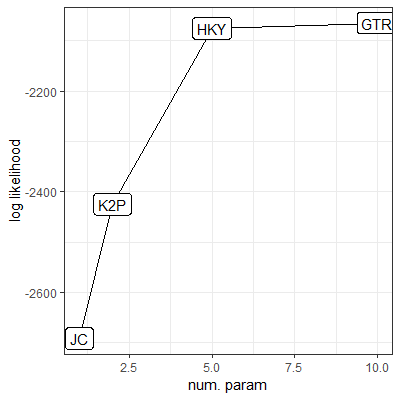
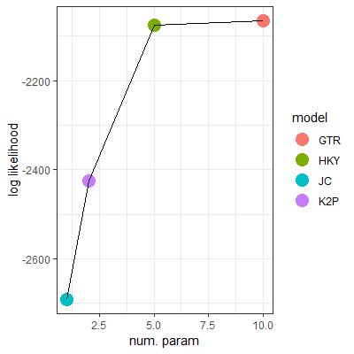
- The two graphs show the log likelihoods (i.e., goodness of fit, or Prob(Data|Model)) of four nucleotide-substitution models for describing patterns of Human/Chimp DNA sequence divergence
- Reproduce (with proper axis labels and custom size and shape for the points) one of the graphs using R/ggplot2. Read the data set using
lk <- read_csv("http://diverge.hunter.cuny.edu/~weigang/lk.csv")
- Explain why HKY is the best model for the data
|
|
|
- 11/11 (M).
- Tree Testing (Chapter 5, pages 194-198).
- 11/14 (TH).
- Review exercises (Chapter 5, pages 207-209) .
- 11/18 (M). 3rd Mid-term exam
Part 4. Mechanisms of molecular evolution
- 11/21 (TH).
- Mechanism of molecular evolution: Overview (pages 35-38) & Rates of nucleotide substitutions (pages 111-125).
- 11/25 (M). In-class computer exercise:
- Ka/Ks test of natural selection (pg 116-124). In-class exercise
| Final project (20 pts). Due: 12/9, Monday)
|
- Calculate genetic distances
- Download or Copy/Paste the lizard DNA sequences to your own computer and save the file as "anoles.txt" in a directory (e.g., "Document")
- Align the DNA sequences using this website and save the aligned DNA file ("Output->Alignment in Fasta format") as "anoles-aligned.txt" (No need to print or submit the above two DNA sequence files; save them in a folder, e.g., "Document")
- Download & load library: library(ape)
- In RStudio, set working directory to the same one containing alignemnt ("Session" -> "Set Working Directory" -> "Choose Directory")
- Read alignment: mt <- read.FASTA("anoles-aligned.txt")
- Calculate raw distance: mt.raw <- dist.dna(mt, model = "raw")
- Apply Juke-Cantor (one-parameter model) correction: mt.jc <- dist.dna(mt, model = "JC")
- Apply Kimura(two-parameter model, for Ts and Tv) correction: mt.k80 <- dist.dna(mt, model = "K80") to
- Plot JC distance vs the raw distance: plot(mt.raw, mt.jc, xlab = "uncorrected distance (diff/site)", ylab = "corrected distance (sub/site)", xlim = c(0,0.4), ylim = c(0,0.5), las =1)
- Add a 1:1 line: abline(0,1, col = "red")
- Add K80 distances: points(mt.raw, mt.k80, pch = 3, col = "blue")
- Add a legend: legend(0.05, 0.45, legend = c("JC (1-parameter)", "K80 (2-parameter)"), pch = c(1,3), col = c("black","blue"), bty = "n")
- Export an PDF and print a copy
- Use the graph to explain
- (1) Why it is necessary to correct for raw distances when comparing sequences from distantly related species;
- (2) What is the key difference between the K80 and JC models
- Comparison of distance and parsimony trees (review previous assignments for detailed R-Studio instructions)
- In R studio, install & load the "ape" and "phangorn" libraries
- Obtain a neighbor-joining tree using K80 model: tree.nj <- NJ(mt.k80)
- Plot a midpoint rooted tree: plot(midpoint(tree.nj))
- Add a scale bar: add.scale.bar()
- Print tree and answer this question: what does the distance represent? What is the unit?
- Obtain a maximum parsimony tree
- Convert object to a different class: aln.phy <- as.phyDat(mt)
- Search maximum parsimony tree.mp <- optim.parsimony(tree.nj, aln.phy)
- Get tree distance: tree.mp <- acctran(tree.mp, aln.phy)
- Plot tree: plot(midpoint(tree.mp))
- Add a scale bar: add.scale.bar()
- Print tree and answer the question: what does the distance represent? What is the unit?
- Compare the two trees and explain the differences in these two methods: Which one uses full sequence information and why?
- Bootstrap analysis
- aln.fas <- read.dna("anoles-aligned.txt", format ="fasta")
- Create a function for re-rooted distance tree: tree.fun <- function(x) root(nj(dist.dna(x)), outgroup = c("Leiocephalus_barahonensis"), resolve.root = T)
- Calculate a tree: tr <- tree.fun(aln.fas)
- Perform bootstrap for 100 pseudo-replicates: boot.trees <- boot.phylo(tr, aln.fas, tree.fun, B=100, rooted =T)
- Plot tree: plot(tr, no.margin = T)
- Add bootstrap values as node labels: nodelabels(boot.trees, bg= "white")
- Explain (1) Does bootstrap test for tree precision or tree accuracy? (2) What does a bootstrap value of 80% mean?
|
- 12/2 (M). SNP statistics & gene frequency analysis: In-class exercises.
- 12/5 (TH) Genetic Drift (pages 47-49). Lecture slides:
- 12/9 (M). (Last Lecture) Review & Course evaluations. Final review slides:
- Dec 16 (Monday) 4-6pm: Comprehensive Final Exam


