Biol425 2015: Difference between revisions
imported>Weigang |
imported>Weigang m (→Useful Links) |
||
| (85 intermediate revisions by the same user not shown) | |||
| Line 77: | Line 77: | ||
{| class="wikitable sortable mw-collapsible" | {| class="wikitable sortable mw-collapsible" | ||
|- style="background-color:lightsteelblue;" | |- style="background-color:lightsteelblue;" | ||
! Assignment #2 (<font color="red"> | ! Assignment #2 (<font color="red">Finalized as of Saturday 2/7/205, at 1pm</font>) | ||
|- style="background-color:powderblue;" | |- style="background-color:powderblue;" | ||
| '''UNIX Exercises''' (10 pts)<br> | | '''UNIX Exercises''' (10 pts)<br> | ||
| Line 86: | Line 86: | ||
# Use the <code>long-orf</code> command to predict ORFs on the mystery_seq1. Save resulting coord file as "mystery_seq1.coord". | # Use the <code>long-orf</code> command to predict ORFs on the mystery_seq1. Save resulting coord file as "mystery_seq1.coord". | ||
# Extract ONLY the lines containing ORF information into a new file "mystery_seq1.coord2" using <code>grep</code> | # Extract ONLY the lines containing ORF information into a new file "mystery_seq1.coord2" using <code>grep</code> | ||
# Run <code>extract</code> to extract FASTA sequences of all predicted ORFs | # Run <code>extract</code> to extract FASTA sequences of all predicted ORFs. Save as "mys.nuc". | ||
# Use <code>bioseq</code> to | # Translate "mys.nuc" with <code>bioseq -t1</code>. Save to "mys.pep" (don't be surprised if the 2nd sequence contains internal stop codons) | ||
Note: Show all commands and outputs. | # Use <code>bioseq</code> to extract the ORF sequences, save as "mys.nuc2" | ||
# Translate "mys.nuc2" with <code>bioseq -t1</code>. Save to "mys.pep2". This file should NOT contain any internal stop codons. | |||
Note: Show all commands and outputs.To log off, type "exit" twice (first log out of the "cslab" host, 2nd time log off the "eniac" host). | |||
|} | |} | ||
---- | ---- | ||
===February 11. Genomics (2): BioPerl=== | ===February 11. Genomics (2): BASH & BLAST=== | ||
* Lecture Slides | * Lecture Slides: [[File:Session-3-small-2015.pdf|thumbnail]] | ||
* Learning goal: (1) BASH scripting; (2) Homology searching with NCBI blast | |||
* In-Class exercises | |||
# Build workflow with BASH scripts | |||
<syntaxhighlight lang=bash"> | |||
#!/usr/bin/bash | |||
bioseq -s"163,1272" cp9.plasmid.fas > gene-0001.nuc; | |||
bioseq -t1 gene-0001.nuc > gene-0001.pep; | |||
exit; | |||
</syntaxhighlight> | |||
Save the above as "extract-gene-v1.bash". Make it executable with <code>chomd +x extract-gene-v1.bash</code>. Run it with <code>./extract-gene-v1.bash</code> | |||
# Improvement 1. make it work for other genes (by using variables) | |||
<syntaxhighlight lang=bash"> | |||
#!/usr/bin/bash | |||
id=$1; | |||
begin=$2; | |||
end=$3; | |||
bioseq -s"$begin,$end" cp9.plasmid.fas > gene-$id.nuc; | |||
bioseq -t1 gene-$1.nuc > gene-$id.pep; | |||
exit; | |||
</syntaxhighlight> | |||
Save the above as "extract-gene-v2.bash". Make it executable with <code>chomd +x extract-gene-v2.bash</code>. Run it with <code>./extract-gene-v2.bash 0001 163 1272</code> (Note three arguments). Question: How to modify the code to make it work for genes encoded on the reverse strand? | |||
# Improvement 2. make it work for both positive and negative genes (by using an "if" statement) | |||
<syntaxhighlight lang=bash"> | |||
#!/usr/bin/bash | |||
id=$1; | |||
begin=$2; | |||
end=$3; | |||
strand=$4; | |||
bioseq -s"$begin,$end" cp9.plasmid.fas > gene-$id.nuc; | |||
if [ $strand -gt 0 ]; then | |||
bioseq -t1 gene-$1.nuc > gene-$id.pep; | |||
else | |||
bioseq -r gene-$1.nuc > gene-$id.rev; | |||
bioseq -t1 gene-$1.rev > gene-$id.pep; | |||
fi; | |||
exit; | |||
</syntaxhighlight> | |||
# Improvement 3. Make it read "cp9.coord" as an input file, by using a "while" loop: | |||
<syntaxhighlight lang=bash"> | |||
#!/usr/bin/bash | |||
cat $1 | grep "^[0-9]" | while read line; do | |||
id=$(echo $line | cut -f1 -d' '); # run commands and save result to a variable | |||
x1=$(echo $line | cut -f2 -d' '); | |||
x2=$(echo $line | cut -f3 -d' '); | |||
strand=$(echo $line | cut -f4 -d' '); | |||
if [ $strand -lt 0 ]; then | |||
bioseq -s"$x2,$x1" cp9.plasmid.fas > gene-$id.nuc; | |||
bioseq -r gene-$id.nuc > gene-$id.rev; | |||
bioseq -t1 gene-$id.rev; | |||
else | |||
bioseq -s"$x1,$x2" cp9.plasmid.fas > gene-$id.nuc; | |||
bioseq -t1 gene-$id.nuc; | |||
fi; | |||
done; | |||
exit; | |||
</syntaxhighlight> | |||
# Run Stand-alone BLAST: | |||
* Add blast binaries to your $PATH in ".bash_profile": export PATH=$PATH:/data/biocs/b/bio425/ncbi-blast-2.2.30+/bin/ | |||
* BLAST tutorial 1. A single unknown sequence against a reference genome | |||
<syntaxhighlight lang=bash" line enclose="div"> | |||
cp ../../bio425/data/GBB.pep ~/. # Copy the reference genome | |||
cp ../../bio425/data/unknown.pep ~/. # Copy the query sequence | |||
makeblastdb -in GBB.pep -dbtype prot -parse_seqids -out ref # make a database of reference genome | |||
blastp -query unknown.pep -db ref # Run simple protein blast | |||
blastp -query unknown.pep -db ref -evalue 1e-5 # filter by E values | |||
blastp -query unknown.pep -db ref -evalue 1e-5 -outfmt 6 # concise output | |||
blastp -query unknown.pep -db ref -evalue 1e-5 -outfmt 6 | cut -f2 > homologs-in-ref.txt # save a list of homologs | |||
blastdbcmd -db ref -entry_batch homologs-in-ref.txt > homologs.pep # extract homolog sequences | |||
</syntaxhighlight> | |||
* In-Class challenges | |||
{| class="wikitable sortable mw-collapsible" | |||
|- style="background-color:lightsteelblue;" | |||
! Assignment #3 <font color="red">(Finalized on Feb 15, 2015, 2AM)</font> | |||
|- style="background-color:powderblue;" | |||
| '''BASH Exercises''' (20 pts)<br> | |||
Note: Log on your eniac account and then ssh into a "cslab" host (e.g., ssh cslab5). Perform the following tasks without changing directory (i.e., stay in your home directory). | |||
# UNIX filter exercises (5 pts) | |||
## For the codon file <code>/data/biocs/b/bio425/data/codon.table.T</code>, sort by single-letter code of amino acids | |||
## use "grep" to show only codons that start with an "A" | |||
## Show all codons for "Arg", without amino acid symbols | |||
## Use an editor, compose a BASH script (name it "read-codon.bash") that uses a "while" loop to read each line of this file. First, use "grep -v" to exclude stop codons. Then, create three variables to capture the values of three elements on each line. For each line, print the output in the following format: "AAA codes for Lys (K)". | |||
# Exercise for the use of wildcard & BASH "for" loop (5 pts) | |||
## Long-list (i.e., ls -l) the following file in the "/data/biocs/b/bio425/data/GBB.1con-splitted/" directory: Borrelia_burgdorferi_3615_main.fas (this file contains the main chromosome sequence of the B31 strain of Lyme disease bacteria). Run <code>bioseq -l</code> to find out the length of this sequence. | |||
## Without changing directory, long-list ALL files with the ".fas" suffix in the same directory (using wildcard). This command list all replicons (chromosome and 21 plasminds) of this genome. | |||
## Write a BASH "for" loop on the command line (do not use an editor) to obtain length of each replicon using <code>bioseq -l</code> | |||
# Exercise for BASH script (5 pts): Compose a pipeline of predicting and extracting gene sequences using a single BASH script. (You may name this script "predict-orfs.bash"). The script takes a genome sequence file as a single input. It outputs predicted ORF sequences in two files: "orf.nuc" & "orf.pep". Copy <code>../../bio425/data/GBB.1con-splitted/Borrelia_burgdorferi_4091_cp26_plasmid_B.fas</code> file to your home directory and predict all ORFs on this plasmid. Note your resulting "orf.pep" file should not contain any stop codons except as the last. | |||
# BLAST exercise (5 pts). | |||
## Use "blastp" to identify matches of the sequence <code>../../bio425/data/unknown.pep</code> in the "ref" database (which was created in class), using an e-value cutoff of 1e-10 | |||
## Show all pairwise alignments | |||
## Show output in a tabular format (using "-outfmt 6") | |||
## Explain the following blast terms: "Identity", "Positives", and "Expect". [Hint, visit [http://blast.ncbi.nlm.nih.gov/ the NCBI BLAST home page] and [http://blast.ncbi.nlm.nih.gov/Blast.cgi?CMD=Web&PAGE_TYPE=BlastDocs&DOC_TYPE=FAQ#expect this FAQ]]. | |||
|} | |||
===February 18. No Class (Monday Schedule)=== | |||
===February 25. Genomics (3). Genome BLAST & BioPerl=== | |||
* Lecture Slides: [[File:Session-4-small-2015.pdf|thumbnail]] | |||
* Learning goals: Homology, BLAST, & Object-oriented programming with Perl | |||
* BLAST tutorial 2. Find homologs within the new genome itself | |||
<syntaxhighlight lang=bash" line start=9 enclose="div"> | |||
cp ../../bio425/data/N40.pep ~/. # Copy the unknown genome | |||
makeblastdb -in N40.pep -dbtype prot -parse_seqids -out N40 # make a database of the new genome | |||
blastp -query unknown.pep -db N40 -evalue 1e-5 -outfmt 6 | cut -f2 > homologs-in-N40.txt # find homologs in the new genome | |||
blastdbcmd -db N40 -entry_batch homologs-in-N40.txt >> homologs.pep # append to homolog sequences | |||
</syntaxhighlight> | |||
* BLAST tutorial 3. Multiple alignment & build a phylogeny | |||
<syntaxhighlight lang=bash" line start= 13 enclose="div"> | |||
../../bio425/bin/muscle -in homologs.pep -out homologs.aln # align sequences | |||
cat homologs.aln | tr ':' '_' > homologs2.aln | |||
../../bio425/bin/FastTree homologs2.aln > homologs.tree # build a gene tree | |||
../../bio425/figtree & # view tree (works only in the lab; install your own copy if working remotely) | |||
</syntaxhighlight> | |||
{| class="wikitable sortable mw-collapsible" | |||
|- style="background-color:lightsteelblue;" | |||
! Assignment #4 (Finalized on 2/28/2015, 11am) | |||
|- style="background-color:powderblue;" | |||
| '''BLAST exercise''' (5 pts)<br> | |||
Run BLASTp to identify all homologs of BBA18 in the reference genome ("ref"). | |||
# Obtain BBA18 peptide sequence using <code>blastdbcmd -db ref -entry 'BBA18'</code>. | |||
# Run blastp against the "ref" database with the following e-value cutoffs: 1e-5, 1e-3, and 1e-1. Submit the results for 1e-3 with the "-outfmt 6" option. | |||
# Extract all homologs using <code>blastdbcmd</code> | |||
# Combine all sequences with <code>cat</code> and align all sequences using <code>muscle</code>. Show alignment. | |||
# Build a tree of homologs using <code>FastTree</code>. Display tree with [http://www.evolgenius.info/evolview/ evolview]. | |||
|-style="background-color:powderblue;" | |||
| '''Perl exercise''' (5 pts)<br> | |||
# Compose a Perl script ("dump-coords.pl"), which uses an array (@genes) to hold information for two genes in the <code>../../bio425/data/mys.coord2</code> file. Each element of the array would be a reference to a hash. The hash reference itself would hold gene information in the following format: e.g., <code>$gene={'id'=>'0001', 'start'=>16, 'end'=>324, 'frame'=>'+1', 'score'=>0.929}</code>. Print the array by using the <code>Dumper</code> function. | |||
# Write a 2nd version of the the script ("read-coords.pl"). This time, instead of hard-coding gene information within the code, the script will read the <code>../../bio425/data/mys.coord</code> file, save gene features into variables, and dump the same results. The following code helps you to get started: | |||
<syntaxhighlight lang=perl" enclose="div"> | |||
#!/usr/bin/perl | |||
use strict; | |||
use warnings; | |||
use Data::Dumper; # print complex data structure | |||
# ---------------------------------------- | |||
# Author : WGQ | |||
# Date : February 30, 2015 | |||
# Description : Read coord file | |||
# Input : A coord file | |||
# Output : Coordinates and read frame for each gene | |||
# ---------------------------------------- | |||
die "Usage: $0 <coord_file>\n" unless @ARGV == 1; # print usage | |||
my @genes; # declare the array | |||
while(<>) { # read file from argument | |||
my $line = $_; # save each line to a variable | |||
next unless $line =~ /^\d+/; # skip lines except those reporting genes | |||
<Your code: split the $line on white spaces and save into variables> | |||
<Your code: construct anonymous hash and push into @genes> | |||
} | |||
print Dumper(\@genes); | |||
exit; | |||
</syntaxhighlight> | |||
|} | |||
===March 4: Genomics (4). Object-oriented Perl (Continued) === | |||
* Lecture Slides: [[File:Session-5-Spring-2015-small.pdf|thumbnail|Session 3]] | |||
* Learning goal: (1) Object-Oriented Perl; (2) BioPerl | * Learning goal: (1) Object-Oriented Perl; (2) BioPerl | ||
* In-Class Exercises | * In-Class Exercises | ||
| Line 142: | Line 298: | ||
{| class="wikitable sortable mw-collapsible" | {| class="wikitable sortable mw-collapsible" | ||
|- style="background-color:lightsteelblue;" | |- style="background-color:lightsteelblue;" | ||
! Assignment # | ! Assignment #5 (<font color="red">Finalized on March 6th, 2015, 10pm</font>) | ||
|- style="background-color:powderblue;" | |- style="background-color:powderblue;" | ||
| '''BioPerl exercises'''<br /> | | '''BioPerl exercises (10 pts)'''<br /> | ||
# | # Write an "extract.pl" using Perl & BioPerl that extract coding sequences from "coord" files. The script will use Bio::SeqIO to read the genome FASTA file ("mystery_seq1.fas", see Assignment #2 above). It will also read the "mystery_seq1.coord" (see Assignment #2 above) as the 2nd argument. Use Bio::Seq to obtain coding sequences and translate sequences. Your output of protein sequences should not contain stop codons except as the last codon. The following template helps you get started: | ||
<syntaxhighlight lang="perl" line enclose="div"> | <syntaxhighlight lang="perl" line enclose="div"> | ||
#!/usr/bin/perl | #!/usr/bin/perl | ||
| Line 156: | Line 311: | ||
# File : extract.pl | # File : extract.pl | ||
# Author : WGQ | # Author : WGQ | ||
# Date : | # Date : March 5, 2015 | ||
# Description : Emulate glimmer EXTRACT program | # Description : Emulate glimmer EXTRACT program | ||
# Input : A FASTA file with 1 DNA seq and coord file from LONG-ORF | # Input : A FASTA file with 1 DNA seq and coord file from LONG-ORF | ||
| Line 163: | Line 318: | ||
die "Usage: $0 <FASTA_file> <coord_file>\n" unless @ARGV > 0; | die "Usage: $0 <FASTA_file> <coord_file>\n" unless @ARGV > 0; | ||
my ($fasta_file, $coord_file) = @ARGV; | my ($fasta_file, $coord_file) = @ARGV; | ||
my $ | my $fasta_input = Bio::SeqIO->new(<your code>); # create a file handle to read sequences from a file | ||
my $output = Bio::SeqIO->new(-file=>">$fasta_file".".out", -format=>'fasta'); # create a file handle to output sequences into a file | my $output = Bio::SeqIO->new(-file=>">$fasta_file".".out", -format=>'fasta'); # create a file handle to output sequences into a file | ||
my $seq_obj = $input->next_seq(); | my $seq_obj = $input->next_seq(); # get sequence object from FASTA file | ||
# Read COORD file & extract sequences | # Read COORD file & extract sequences | ||
open COORD, "<" . $coord_file; | open COORD, "<" . $coord_file; | ||
while (<COORD>) { | while (<COORD>) { | ||
my $line = $_; | |||
chomp $line; | |||
next unless $line =~ /^\d+/; # skip lines except | |||
my ($seq_id, $cor1, $cor2, $strand, $score) = split /\s+/, $line; # split line on white spaces | |||
if (<your code: if strand is positive>) { | |||
<your code: use trunc function to get sub-sequence as an object> | |||
} else { | |||
<your code: use the trunc() function to get sub-sequence as an object> | |||
<your code: use the revcom() function to reverse-complement the seq object> | |||
} | |||
<your code: use translate() function to obtain protein sequence as an abject, "$pro_obj"> | |||
$output->write_seq($pro_obj); | |||
} | } | ||
close COORD; | close COORD; | ||
exit; | exit; | ||
</syntaxhighlight> | </syntaxhighlight> | ||
|} | |} | ||
===March 11: | ===March 11: Review === | ||
* Review: [[File:Session-6- | * Review slides: [[File:Session-6-reviw-sp-15.pdf|thumbnail]] | ||
* | * Practice Tests | ||
# Browse & Filter "Big Data" files with UNIX filters | |||
## Genome file | |||
### List all FASTA files in the "../../bio425/data" directory: <code>ls ../../bio425/data/*.fas</code> | |||
### Count number of sequences in a FASTA file: "../../bio425/data/GBB.pep": <code>grep -c ">" ../../bio425/data/GBB.pep</code> | |||
### Count number of sequences in all FASTA file in this directory: <code>grep -c ">" ../../bio425/data/*.fas</code> | |||
### Remove directory names from the above output: <code>grep ">" ../../bio425/data/*.fas | sed 's/^.\+data\///'</code> or <code>grep ">" ../../bio425/data/*.fas| cut -f5 -d'/'</code> | |||
## GenBank file | |||
### Show top 10 lines in "../../bio425/data/mdm2.gb": <code>head ../../bio425/data/mdm2.gb</code> | |||
### Show bottom 10 lines: <code>tail ../../bio425/data/mdm2.gb</code> | |||
### Extract all lines containing nucleotides: <code>cat ../../bio425/data/mdm2.gb | grep -P "^\s+\d+[atcg\s]+$"</code> | |||
## Transcriptome file: a microarray data set | |||
### Count the number of lines in "../../bio425/data/ge.dat": <code>wc -l ../../bio425/data/ge.dat</code> | |||
### Count the number of genes: <code>cut -f1 ../../bio425/data/ge.dat | grep -vc "Desc"</code> | |||
### Count the number of cells: <code>head -1 ../../bio425/data/ge.dat | tr '\t' '\n' | grep -vc "Desc"</code> | |||
## Transcriptome file: an RNA-SEQ output file | |||
### Count the nubmer of lines in "../../bio425/data/gene_exp.diff": <code>wc -l ../../bio425/data/gene_exp.diff</code> | |||
### Show head: <code>head ../../bio425/data/gene_exp.diff</code> | |||
### Show tail: <code>tail ../../bio425/data/gene_exp.diff</code> | |||
### Count nubmer of "OK" gene pairs (valid comparisons): <code>grep -c "OK" ../../bio425/data/gene_exp.diff</code> | |||
### Count nubmer of significantly different genes: <code>grep -c "yes$" ../../bio425/data/gene_exp.diff</code> | |||
### Sort by "log2(fold_change)": <code>grep "yes$" ../../bio425/data/gene_exp.diff | cut -f1,10 | sort -k2 -n</code> | |||
## A proteomics dataset: SILAC | |||
### Count the number of line in "../../bio425/data/Jill-silac-batch-1.dat": <code>wc -l ../../bio425/data/Jill-silac-batch-1.dat</code> | |||
### Show top: <code>head ../../bio425/data/Jill-silac-batch-1.dat</code> | |||
### Show bottom: <code>wc -l ../../bio425/data/Jill-silac-batch-1.dat</code> | |||
### Show results for P53 genes: <code>grep -w "TP53" ../../bio425/data/Jill-silac-batch-1.dat</code> | |||
### Sort by "log_a_b_ratio": <code>sort -k5 -n ../../bio425/data/Jill-silac-batch-1.dat</code> | |||
### Show ranking of P53: <code>sort -k5 -n -r ../../bio425/data/Jill-silac-batch-1.dat | cat -n | grep -w "TP53"</code> | |||
# Identify homologs and build a phylogeny | |||
## Copy genome file: "../../bio425/data/GBB.1con-splitted/Borrelia_burgdorferi_4075_lp54_plasmid_A.fas" to your home directory as "lp54.fas": <code>cp ../../bio425/data/GBB.1con-splitted/Borrelia_burgdorferi_4075_lp54_plasmid_A.fas lp54.fas</code> | |||
## Identify ORFs in file using "long-orfs": <code>long-orfs lp54.fas lp54.coord</code> | |||
## Extract nucleotide sequences: <code>extract lp54.fas lp54.coord > lp54.nuc</code> | |||
## Use "bioseq" to translate into peptides, into "lp54.pep": <code>bioseq -t1 lp54.nuc > lp54.pep</code> | |||
## Make a blast database: <code>makeblastdb -in lp54.pep -dbtype 'prot' -parse_seqids -out lp54</code> | |||
## Copy file "../../bio425/data/BBA68.pep" to your home directory: <code>cp ../../bio425/data/BBA68.pep .</code> | |||
## Find homologs of "BBA68.pep" in "lp54.pep" using "blastp": <code>blastp -query BBA68.pep -db lp54 -evalue 1e-5 -outfmt 6 | cut -f2 > BBA68.homologs</code> | |||
## Extract all blast homologs using "blastdbcmd": <code>blastdbcmd -db lp54 -entry_batch BBA68.homologs > BBA68.homologs.pep</code> | |||
## Align all homologs using "muscle": <code>muscle -in BBA68.homologs.pep -out BBA68.homologs.aligned</code> | |||
## Build a tree of BBA65 homologs using "FastTree": <code>FastTree BBA68.homologs.aligned > BBA68.dnd</code> | |||
## Show tree with [http://www.evolgenius.info/evolview/ evolview] | |||
# Review BASH "while" & "for" loops (see Assignment #3) | |||
# Review the use Bio::SeqIO to read FASTA files and the use Bio::Seq methods to manipulate sequences (see Assignment #5) | |||
===March 18. Midterm Practicum=== | ===March 18. Midterm Practicum=== | ||
10:10-12 | # Hours: 10:10-12:30pm | ||
# Rules: Computer access to course wiki & terminal only. | |||
# Copy and paste commands and outputs to a text file | |||
===March 25 (No Class; Do Assignment #6)=== | ===March 25 (No Class; Do Assignment #6)=== | ||
{| class="wikitable sortable mw-collapsible" | {| class="wikitable sortable mw-collapsible" | ||
|- style="background-color:lightsteelblue;" | |- style="background-color:lightsteelblue;" | ||
! Assignment #6 (Finalized on | ! Assignment #6 (Finalized on Tuesday 3/24/2015, 11pm) | ||
|-style="background-color:powderblue;" | |-style="background-color:powderblue;" | ||
| '''Perl/BioPerl Exercises''' ( | | '''Perl/BioPerl Exercises''' (10 pts)<br> | ||
* The following Perl code dumps nucleotide and codon frequencies given a coding sequence. It is based on the [http://search.cpan.org/~cjfields/BioPerl-1.6.923/Bio/Tools/SeqStats.pm Bio::Tools::SeqStats module of BioPerl]. Copy and run it with <code>./seq-stats.pl ../../bio425/data/B31_ospA.fas</code> to understand its behavior. | * The following Perl code dumps nucleotide and codon frequencies given a coding sequence. It is based on the [http://search.cpan.org/~cjfields/BioPerl-1.6.923/Bio/Tools/SeqStats.pm Bio::Tools::SeqStats module of BioPerl]. Copy and run it with <code>./seq-stats.pl ../../bio425/data/B31_ospA.fas</code> to understand its behavior. | ||
<syntaxhighlight lang=perl line enclose="div"> | <syntaxhighlight lang=perl line enclose="div"> | ||
| Line 336: | Line 421: | ||
** Write a subroutine named as "count_monomers" to count and print the frequency of each nucleotide (in percentage), sorted by nucleotide type. The argument for the subroutine would be the sequence as a string, as in <code>count_monomers($seqobj->seq)</code>. The return value would be a reference to a hash (the same as the <code>$monomers</code> in the above code). | ** Write a subroutine named as "count_monomers" to count and print the frequency of each nucleotide (in percentage), sorted by nucleotide type. The argument for the subroutine would be the sequence as a string, as in <code>count_monomers($seqobj->seq)</code>. The return value would be a reference to a hash (the same as the <code>$monomers</code> in the above code). | ||
** Hint: use hash to count unique bases, see [http://my.safaribooksonline.com/book/programming/perl/1565922433/arrays/ch04-13496#X2ludGVybmFsX0h0bWxWaWV3P3htbGlkPTEtNTY1OTItMjQzLTMlMkZjaDA0LTE3NDIxJnF1ZXJ5PQ== Perl Cookbook example], especially the code listed under "4.6.2.4. Faster but different" | ** Hint: use hash to count unique bases, see [http://my.safaribooksonline.com/book/programming/perl/1565922433/arrays/ch04-13496#X2ludGVybmFsX0h0bWxWaWV3P3htbGlkPTEtNTY1OTItMjQzLTMlMkZjaDA0LTE3NDIxJnF1ZXJ5PQ== Perl Cookbook example], especially the code listed under "4.6.2.4. Faster but different" | ||
* In a similar way, write a subroutine named as "count_codons" to count and print the frequency of each ''codon'', sorted by codons. Your codon counts should be the same as those produced by the listed code. | |||
|} | |} | ||
| Line 354: | Line 429: | ||
* R Tutorial 1 | * R Tutorial 1 | ||
# Set a working directory | # Set a working directory | ||
## Using a Linux terminal, make a directory called <code>R-work</code> | ## Using a Linux terminal, make a directory called <code>R-work</code>, "cd" into this directory. | ||
## Start R: <code>Type " | ## Start R studio: <code>Type "rstudio &" on terminal prompt and hit return</code> ('''Note: This link works only if you use computers in the 1000G lab. Install and use your own R & R Studio for homework assignments''') | ||
## Find working directory with <code>getwd()</code> | ## Find working directory with <code>getwd()</code> | ||
# The basic R data structure: Vector | # The basic R data structure: Vector | ||
## Construct a character vector with <code>c.vect=c("red", "blue", "green", "orange", "yellow", "cyan")</code> | ## Construct a character vector with <code>c.vect=c("red", "blue", "green", "orange", "yellow", "cyan")</code> | ||
| Line 379: | Line 453: | ||
## Descriptive statistics: <code>sum(n.vect); var(n.vect); sd(n.vect)</code> | ## Descriptive statistics: <code>sum(n.vect); var(n.vect); sd(n.vect)</code> | ||
## Sort: <code>order(n.vect)</code>. How would you get an ordered vector of n.vect? [Hint: use <code>?order</code> to find the return values] | ## Sort: <code>order(n.vect)</code>. How would you get an ordered vector of n.vect? [Hint: use <code>?order</code> to find the return values] | ||
## | ## Arithmetic: <code>n.vect +10; n.vect *10; n.vect / 10</code> | ||
# Quit an R session | # Quit an R session | ||
## Click on the "History" tab to review all your commands | ## Click on the "History" tab to review all your commands | ||
| Line 385: | Line 459: | ||
## Save all your data to a default file '''.RData''' and all your commands to a default file ".Rhistory" with <code>save.image()</code> | ## Save all your data to a default file '''.RData''' and all your commands to a default file ".Rhistory" with <code>save.image()</code> | ||
## Quit R-Studio with <code>q()</code> | ## Quit R-Studio with <code>q()</code> | ||
* R tutorial 2 | * R tutorial 2. Data distribution using histogram | ||
# Start a new R studio session and set working directory to <code>~/R-work</code> | # Start a new R studio session and set working directory to <code>~/R-work</code> | ||
# Generate a vector of 100 normal deviates using <code>x.ran=rnorm(100)</code> | # Generate a vector of 100 normal deviates using <code>x.ran=rnorm(100)</code> | ||
| Line 393: | Line 467: | ||
# Test if the data points are normally distributed.[Hints: use qqnorm() and qqline()] | # Test if the data points are normally distributed.[Hints: use qqnorm() and qqline()] | ||
# Save a copy of your plot using "Export"->"Save Plot as PDF" | # Save a copy of your plot using "Export"->"Save Plot as PDF" | ||
* R tutorial 3 | * R tutorial 3. Matrix & Data Frames | ||
# Using a Linux terminal, make a copy of breast-cancer transcriptome file <code>/data/biocs/b/bio425/data/ge.dat</code> in your R working directory | # Using a Linux terminal, make a copy of breast-cancer transcriptome file <code>/data/biocs/b/bio425/data/ge.dat</code> in your R working directory | ||
# Start a new R studio session and set working directory to <code>~/R-work</code> | # Start a new R studio session and set working directory to <code>~/R-work</code> | ||
| Line 407: | Line 481: | ||
{| class="wikitable sortable mw-collapsible" | {| class="wikitable sortable mw-collapsible" | ||
|- style="background-color:lightsteelblue;" | |- style="background-color:lightsteelblue;" | ||
! Assignment #7 (Finalized on | ! Assignment #7 (Finalized on Friday, April 3, 2015, 3pm) | ||
|- style="background-color:powderblue;" | |- style="background-color:powderblue;" | ||
| | | | ||
* (5 pts) Test the "GT-AG" rule of introns. Complete the following script to extract all intron sequences from this file <code>../../bio425/data/mdm2.gb</code>. | |||
** After carefully studying and deciphering the script, replace "?"s (a total of 6) in the script with real numbers | |||
** Save the script as "splice.pl" & run with the four options individually, as in <code>splice -i mdm2.gb</code>. | |||
** Make a [http://weblogo.berkeley.edu/ SeqLogo] to show that all introns start with "GT" and ends with "AG". To do so, copy & paste individual sequences at the donor sites [http://weblogo.threeplusone.com/create.cgi into this text box] and click "Create Logo". Print and hand in the resulting image file. Indicate which sites are conserved. | |||
** Repeat for the acceptor-site sequences. Indicate which sites are conserved. | |||
<syntaxhighlight lang=perl line enclose="div"> | |||
#!/usr/bin/perl -w | |||
use strict; | |||
use lib '/data/biocs/b/bio425/bioperl-live'; | |||
use Bio::SeqIO; | |||
use Data::Dumper; | |||
use Getopt::Std; | |||
# ---------------------------------------- | |||
# Author : WGQ | |||
# Date : April 2, 2015 | |||
# Description : Extract intron, exon, and junction sequences | |||
# Input : A GenBank file containing introns | |||
# Output : A Fasta file to feed into WebLogo | |||
# Gene Model : ---exon[i]-donor[i]-intron[i]-acceptor[i]-exon[i+1]-donor[i+1]-intron[i+1]-acceptor[i+1]--- | |||
# ---------------------------------------- | |||
# Part 1. Read 4 options & genbank file | |||
my %opts; | |||
getopts("eida", \%opts); # process options | |||
die "Usage: $0 [-e(xon) -i(ntron) --d(onor) --a(cceptor)] <a GenBank file>\n" unless @ARGV == 1 && ($opts{e} || $opts{i} || $opts{d} || $opts{a}); # print usage if no input file or no options given | |||
my $gb = shift @ARGV; | |||
my $in = Bio::SeqIO->new(-file=>$gb, -format=>'genbank'); | |||
my $seq = $in->next_seq(); | |||
my (@exons, @introns, @donors, @acceptors); # declare arrays as data contains | |||
# Part 2. Extract exon information | |||
foreach my $feat ( $seq->get_SeqFeatures() ) { # loop through each genbank feature | |||
next unless $feat->primary_tag() eq "mRNA"; # skip unless the feature is tagged as "mRNA" | |||
my $location_obj = $feat->location(); # splice coordinates saved as a Bio::Location::Split object | |||
my $exon_id = 1; | |||
foreach my $loc ($location_obj->each_Location) { # access each exon coords object | |||
push @exons, { | |||
'order' => $exon_id++, | |||
'start' => $loc->start, | |||
'end' => $loc->end | |||
}; | |||
} | |||
} | |||
# print Dumper(\@exons); exit; # uncomment to see results of parsed exons | |||
# Part 3. Calcuate intron, donor, acceptor objects | |||
## Extract introns coords: | |||
for (my $i=0; $i<$#exons; $i++) { # for each exon | |||
push @introns, { | |||
'order' => $exons[$i]->{order}, | |||
'start' => $exons[$i]->{end}+1, # intron i starts at (exon i)'s end + 1 | |||
'end' => $exons[$i+1]->{start}-1, # intron i ends at (exon i+1)'s start -1 | |||
}; | |||
} | |||
# print Dumper(\@introns); exit; # uncomment to see introns | |||
## Donor sites (-10 to -1 of an exon and 1-20 of intron) | |||
for (my $i=0; $i<$#exons; $i++) { | |||
push @donors, { | |||
'order' => $exons[$i]->{order}, | |||
'start' => $exons[$i]->{end} - ?, # donor i starts at (exon i)'s -10 to -1 | |||
'end' => $introns[$i]->{start} + ?, # donor i ends at (intron i+1)'s 1 to 20 | |||
}; | |||
} | |||
# print Dumper(\@donors); exit; # uncomment to see donor sequences | |||
## Acceptor sites (-20 to -1 of an intron and 1-10 of exon) | |||
for (my $i=0; $i<$#exons; $i++) { | |||
push @acceptors, { | |||
'order' => $exons[$i]->{order}, | |||
'start' => $introns[$i]->{end} - ?, # acceptor i starts at (intron i)'s -20 to -1 | |||
'end' => $exons[$i+1]->{start} + ?, # acceptor i ends at (exon i+1)'s 1 to 10 | |||
}; | |||
} | |||
# print Dumper(\@acceptors); exit; # uncomment to see acceptor sequences | |||
# Part 4. Output sequences | |||
&print_seq("intron", \@introns) if $opts{i}; | |||
&print_seq("exon", \@exons) if $opts{e}; | |||
&print_seq("donor", \@donors) if $opts{d}; | |||
&print_seq("acceptor", \@acceptors) if $opts{a}; | |||
exit; | |||
sub print_seq { | |||
my ($tag, $ref) = @_; | |||
my @bins = @$ref; | |||
foreach my $bin (@bins) { | |||
my $out = Bio::SeqIO->new(-format=>'fasta'); | |||
my $seq =$seq->trunc(?, ?); | |||
$seq->id($tag . "_" . $bin->{order}); | |||
$out->write_seq($seq); | |||
} | |||
} | |||
</syntaxhighlight> | |||
* (2 pts) Install [http://streaming.stat.iastate.edu/CRAN/ R (choose a binary distribution)] first and then [http://www.rstudio.com/ R Studio] to your home/laptop computer [No need to show any output. I trust you on this.] | * (2 pts) Install [http://streaming.stat.iastate.edu/CRAN/ R (choose a binary distribution)] first and then [http://www.rstudio.com/ R Studio] to your home/laptop computer [No need to show any output. I trust you on this.] | ||
* (4 pts) Make 2 histograms based on the "ge" data set: (a) expression values for a single (any one if fine) selected cell line (cell lines are in columns, using small-sized bins, e.g., "br=100") and (b) expression values for a selected (any one if fine) gene (genes are in rows). Show all R commands and the final plots (label the plot title with cell line or gene name) ['''Notes:''' You need to download a copy of the <code>ge.dat</code> onto your own computer. On Mac, you could run this command: <code>scp your_user_name@eniac.cs.hunter.cuny.edu:ge.dat ge.dat</code>. On Windows, download and install <code>sftp</code> or<code> WinSCP</code> for file transfer from/to your eniac account.] | * (4 pts) Make 2 histograms based on the "ge" data set: (a) expression values for a single (any one if fine) selected cell line (cell lines are in columns, using small-sized bins, e.g., "br=100") and (b) expression values for a selected (any one if fine) gene (genes are in rows). Show all R commands and the final plots (label the plot title with cell line or gene name) ['''Notes:''' You need to download a copy of the <code>ge.dat</code> onto your own computer. On Mac, you could run this command: <code>scp your_user_name@eniac.cs.hunter.cuny.edu:ge.dat ge.dat</code>. On Windows, download and install <code>sftp</code> or<code> WinSCP</code> for file transfer from/to your eniac account.] | ||
* (4 pts) Use the help() and example() functions to learn how to use the which() and grep() functions. Show how to use these two functions, respectively, to display gene expression values for a gene called "ESR1" in the "ge" data set. [Hint: use the rownames() function to obtain gene names of the "ge" data set.] | * (4 pts) Use the help() and example() functions to learn how to use the which() and grep() functions. Show how to use these two functions, respectively, to display gene expression values for a gene called "ESR1" in the "ge" data set. [Hint: use the rownames() function to obtain gene names of the "ge" data set.] | ||
|} | |} | ||
===April 8: No class (Spring Recess)=== | ===April 8: No class (Spring Recess)=== | ||
| Line 461: | Line 633: | ||
{| class="wikitable sortable mw-collapsible" | {| class="wikitable sortable mw-collapsible" | ||
|- style="background-color:lightsteelblue;" | |- style="background-color:lightsteelblue;" | ||
! Assignment #8 (Finalized 4/ | ! Assignment #8 (Finalized on Sunday 4/19/2015 at 11:30pm) | ||
|- style="background-color:powderblue;" | |- style="background-color:powderblue;" | ||
| | | | ||
(10 pts) The following table lists expression levels of a gene measured under an Experimental and a Control conditions, each of which was replicated five times: | |||
* | {| class="wikitable" | ||
|- | |||
! !! Experimental !! Control | |||
|- | |||
| Replicate 1 || 606 || 287 | |||
|- | |||
| Replicate 2 || 441 || 198 | |||
|- | |||
| Replicate 3 || 702 || 366 | |||
|- | |||
| Replicate 4 || 597 || 255 | |||
|- | |||
| Replicate 5 || 888 || 402 | |||
|} | |||
Test significance of gene expressions between the Exp and Ref groups. Show all R commands, test results, & plots. | |||
* Plot a boxplot | |||
* Plot a vertical stripcharts. Why is a stripchart more informative than a boxplot? | |||
* Perform a paired t-test, using the log2 scale. Are gene expression values significantly different between the Exp and Ref groups? | |||
* Plot a scatter plot and add a regression line. Show results of regression analysis, include the R-squared value and the p value. Are the expression levels between the two conditions significantly correlated? | |||
|} | |} | ||
| Line 488: | Line 677: | ||
* Tutorial 2. Test differential gene expressions | * Tutorial 2. Test differential gene expressions | ||
<syntaxhighlight lang="bash" line enclose="div"> | <syntaxhighlight lang="bash" line enclose="div"> | ||
gene=read.table(" | gene=read.table("/data/biocs/b/bio425/data/gene_exp.diff", header=T, sep="\t") | ||
dim(gene) | dim(gene) | ||
head(gene) | head(gene) | ||
| Line 498: | Line 687: | ||
{| class="wikitable sortable mw-collapsible" | {| class="wikitable sortable mw-collapsible" | ||
|- style="background-color:lightsteelblue;" | |- style="background-color:lightsteelblue;" | ||
! Assignment #9 (Finalized 4/ | ! Assignment #9 (Finalized on Friday 4/24/2015 at 2pm) | ||
|- style="background-color:powderblue;" | |- style="background-color:powderblue;" | ||
| | | | ||
* ( | * (5 pts). Filter genes in the "ge.mat" using the "mad" function. Retain the top 50 most-variable genes. Calculate pairwise gene and cell correlation distances. Plot a heatmap. Answer the following questions: | ||
** What does the "mad" function return? What is the biological rationale to use this function to filter genes, before identifying subtypes among cell lines? | |||
** How many major subtypes of cancer cells and subgroups of genes you could identify, respectively? | |||
** Label the genes as two largest groups (Group 1 & 2 Genes). Similarly, label the largest two groups of cell lines as "Group 1" and "Group 2" cells. Explain the expression profiles of Group 1 and Group 2 genes in each subgroup of cells. (e.g., "Group 1 genes are up-regulated in Group 1 Cells and down-regulated in Group 2 Cells". Note that the "yellow" is high in heat color and "red" low). | |||
* (5 pts). Transfer the two RNA-SEQ output files ("genes.fpkm_tracking" and "gene_exp.diff", both in the folder "bio425/data/") to your local computer (using "scp"). Make a histogram of the "C2" sample (use the first file), an MA plot to show differences between "C1" and "C2" in FPKM counts (use the first file), and a volcano plot (use the 2nd file). Show all your R commands. How many genes are significantly different between the two conditions (based on the 2nd file)? | |||
|} | |} | ||
| Line 508: | Line 700: | ||
* Learning goals: (1) SNP analysis (single-locus), (2) haplotype analysis (multiple loci) | * Learning goals: (1) SNP analysis (single-locus), (2) haplotype analysis (multiple loci) | ||
* Lecture slides: [[File:Session-10.pdf|thumbnail]] | * Lecture slides: [[File:Session-10.pdf|thumbnail]] | ||
Tutorial. | Tutorial 1. Extract SNP sites | ||
<syntaxhighlight lang=" | <syntaxhighlight lang="perl" line enclose="div"> | ||
#!/usr/bin/perl | |||
# Author: WGQ | |||
# Description: Examine each alignment site as a SNP or constant | |||
# Input: a DNA alignment | |||
# Output: a haplotypes alignemnt | |||
use strict; | |||
use warnings; | |||
use Data::Dumper; | |||
# | # Part I. Read file and store NTs in a hash (use Bio::AlignIO to read an alignment is better) | ||
my %seqs; # declare a hash as sequence container | |||
my $length; | |||
while (<>) { # read file line by line | |||
my $line = $_; | |||
chomp $line; | |||
next unless $line =~ /^seq/; # skip lines unless it starts with "seq" | |||
my ($id, $seq) = split /\s+/, $line; # split on white spaces | |||
$seqs{$id} = [ (split //, $seq) ]; # id as key, an array of nts as value | |||
$length = length($seq); | |||
} | |||
my %is_snp; # declare a hash to store status of alignment columns | |||
# Part II. Go through each site and report status | |||
for (my $pos = 0; $pos < $length; $pos++) { | |||
my %seen_nt; # declare a hash to get counts of each nt at a aligned position | |||
foreach my $id (keys %seqs) { # collect and count all nts at an aligned site | |||
my $nt = $seqs{$id}->[$pos]; | |||
$seen_nt{$nt}++; | |||
} | |||
my @key_nts = keys %seen_nt; | |||
if (@key_nts > 1) { # a SNP site has more than two nucelotdies | |||
$is_snp{$pos} = 1; | |||
} else { # a constant site | |||
$is_snp{$pos} = 0; | |||
} | |||
} | |||
# Part III. Print haplotypes (i.e., nucleotides at SNP sites for each chromosome) | |||
foreach my $id (keys %seqs) { # for each chromosome | |||
print $id, "\t"; | |||
for (my $pos = 0; $pos < $length; $pos++) { # for each site | |||
next unless $is_snp{$pos}; # skip constant site | |||
print $seqs{$id}->[$pos]; # print nt at a SNP site | |||
} | |||
print "\n"; | |||
} | |||
exit; | |||
</syntaxhighlight> | </syntaxhighlight> | ||
Tutorial 2. Hardy-Weinberg Equilibrium: Calculate expected genotype frequencies | |||
{| class="wikitable sortable mw-collapsible" | {| class="wikitable sortable mw-collapsible" | ||
|- style="background-color:lightsteelblue;" | |- style="background-color:lightsteelblue;" | ||
! Assignment #10 (Finalized on Friday 5/ | ! Assignment #10 (Finalized on Friday 5/1/2015, 1am) | ||
|- style="background-color:powderblue;" | |- style="background-color:powderblue;" | ||
| | | | ||
* | * Based on the <code>../../bio425/data/ex3-1.aln</code>, | ||
* (5 pts). Analyze alignment by eye: Define "allele", "SNP", and "haplotype". Print out the alignment | |||
** Label all SNP sites | |||
** Count frequency of each of the two alleles at the first SNP site | |||
** List all haplotypes, and count frequency of each haplotype. | |||
** How many SNP (i.e., variable) sites you expect to see in a window of DNA containing 10K bases among humans? | |||
** How many nucleotide states (2, 3, or 4) you expect to see for an individual SNP site? | |||
** Do you expect to see more or less transitons than tranvsersions? | |||
** More synonymous or nonsynonymous SNPs (if the sequence codes for a protein)? | |||
* (5 pts). Complete the above PERL script by replacing the two question marks. Compare your output to the haplotypes you obtained manually. They should be the same. | |||
|} | |} | ||
| Line 544: | Line 772: | ||
* Learning goals: Case-Control studies for gene mapping | * Learning goals: Case-Control studies for gene mapping | ||
* Lecture slides: [[File:Session-11-small.pdf|thumbnail]] | * Lecture slides: [[File:Session-11-small.pdf|thumbnail]] | ||
* Tutorial | * Tutorial 1. Test linkage disequilibrium (LD) | ||
* Tutorial 2. Genome-wide association studies (GWAS) | |||
* Tutorial 3. Test of Hardy-Weinberg equilibrium (for random mating & presence of natural selection) | |||
for | |||
===May 13: Final Review=== | ===May 13: Final Review=== | ||
* Review slides: [[File:Final-Review-small.pdf|thumbnail]] | * Review slides: [[File: Final-Review-small-bio425-sp-2015.pdf|thumbnail]] | ||
* | * Tutorial 3. Database access with DBI | ||
* [http://www.hunter.cuny.edu/te '''Teacher's evaluation'''] | * [http://www.hunter.cuny.edu/te '''Teacher's evaluation'''] | ||
* All make-up assignments due May 20. | |||
===May 20: Final Exam=== | ===May 20: Final Exam=== | ||
* Reminder: [http://www.hunter.cuny.edu/te '''Teacher's evaluation'''] | * Reminder: [http://www.hunter.cuny.edu/te '''Teacher's evaluation'''] | ||
| Line 622: | Line 818: | ||
==Useful Links== | ==Useful Links== | ||
* [http://korflab.ucdavis.edu/Unix_and_Perl/current.html An online UNIX & PERL Tutorial for biologiests] | |||
===Unix Tutorials=== | ===Unix Tutorials=== | ||
Latest revision as of 20:20, 25 January 2016
Course Schedule (All Wednesdays)
January 28. Course overview & Unix tools
- Course Overview. Lecture slides:
- Learning Goals: (1) Understand the "Omics" files; (2) Review/Learn Unix tools
- In-Class Tutorial: Unix file filters
- Without changing directory, long-list genome, transcriptome, and proteome files using
ls - Without changing directory, view genome, transcriptome, and proteome files using
less -S - Using
grep, find out the size of Borrelia burgdorferi B31 genome in terms of the number of replicons ("GBB.1con" file) - Using
sort, sort the replicons by (a) contig id (3rd field, numerically); and (b) replicon type (4th field) - Using
cut, show only the (a) contig id (3rd field); (b) replicon type (4th field) - Using
tr, (a) replace "_" with "|"; (b) remove ">" - Using
sed, (a) replace "Borrelia" with abbreviation "B."; (b) remove "plasmid" from all lines - Using
paste -s, extract all contig ids and concatenate them with ";" - Using a combination of
cut and uniq, count how many circular plasmids ("cp") and how many linear plasmids ("lp")
- In-Class Challenges
- Using the "GBB.seq" file, find out the number of genes on each plasmid
grep ">" ../../bio425/data/GBB.seq | cut -c1-4| sort | uniq -c- Using the "ge.dat" file, find out (a) the number of genes; (b) the number of cell lines; (c) the expression values of three genes: ERBB2, ESR1, and PGR
grep -v "Description" ../../bio425/data/ge.dat | wc -l; or:  grep -vc "Description" ../../bio425/data/ge.dat
grep "Description" ../../bio425/data/ge.dat | tr '\t' '\n'| grep -v "Desc" | wc -l
grep -Pw "ERBB2|PGR|ESR1" ../../bio425/data/ge.dat| Assignment #1 |
|---|
Unix Text Filters (10 pts) Show both commands and outputs for the following questions:
|
February 4. Genomics (1): Gene-Finding
- Learning goals: (1) Running UNIX programs; (2) Parse text with Perl anonymous hash
- Lecture slides:
- In-Class Tutorials
- Identify ORFs in a prokaryote genome
- Go to NCBI ORF Finder page
- Paste in the GenBank Accession: AE000791.1 and click "orfFind"
- Change minimum length for ORFs to "300" and click "Redraw". How many genes are predicted? What is the reading frame for each ORF? Coordinates? Coding direction?
- Click "Six Frames" to show positions of stop codons (magenta) and start codons (cyan)
- Gene finder using GLIMMER
- Locate the GLIMMER executables:
ls /data/biocs/b/bio425/bin/ - Locate Borrelia genome files:
ls /data/biocs/b/bio425/data/GBB.1con-splitted/ - Predict ORFs:
../../bio425/bin/long-orfs ../../bio425/data/GBB.1con-splitted/Borrelia_burgdorferi_4041_cp9_plasmid_C.fas cp9.coord[Note the two arguments: one input file and the other output filename] - Open output file with
cat cp9.coord. Compare results with those from NCBI ORF Finder. - Extract lines with coordinates"
grep "^[0-9]" cp9.coord > cp9.coord2 - Extract sequences into a FASTA file:
../../bio425/bin/extract ../../bio425/data/GBB.1con-splitted/Borrelia_burgdorferi_4041_cp9_plasmid_C.fas cp9.coord2 > cp9.fas[Note two input files and standard output, which is then redirected (i.e., saved) into a new file]
- Locate the GLIMMER executables:
- bioseq
- Add
bp-utilsinto $PATH by editing the .bash_profile file and runsource .bash_profile - Run
bioseqwith these options:-l, -n, -c, -r, -t1, -t, -t6, and -s - In-Class Challenge: use
bioseqto extract and translate the 1st (+1 frame) and 5th (-1 frame) genes.
- Add
cp ../../bio425/data/GBB.1con-splitted/Borrelia_burgdorferi_4041_cp9_plasmid_C.fas cp9.plasmid.fas # copy plasmid sequence
bioseq -s'163,1272' cp9.plasmid.fas | bioseq -t1 # extract first predicted ORF (+1 frame)
bioseq -s'3853,4377' cp9.plasmid.fas | bioseq -r | bioseq -t1 # extract 5th ORF (since it is -1 frame, need to rev-com before translation| Assignment #2 (Finalized as of Saturday 2/7/205, at 1pm) |
|---|
UNIX Exercises (10 pts)
Note: Show all commands and outputs.To log off, type "exit" twice (first log out of the "cslab" host, 2nd time log off the "eniac" host). |
February 11. Genomics (2): BASH & BLAST
- Lecture Slides:
- Learning goal: (1) BASH scripting; (2) Homology searching with NCBI blast
- In-Class exercises
- Build workflow with BASH scripts
#!/usr/bin/bash
bioseq -s"163,1272" cp9.plasmid.fas > gene-0001.nuc;
bioseq -t1 gene-0001.nuc > gene-0001.pep;
exit;
Save the above as "extract-gene-v1.bash". Make it executable with chomd +x extract-gene-v1.bash. Run it with ./extract-gene-v1.bash
- Improvement 1. make it work for other genes (by using variables)
#!/usr/bin/bash
id=$1;
begin=$2;
end=$3;
bioseq -s"$begin,$end" cp9.plasmid.fas > gene-$id.nuc;
bioseq -t1 gene-$1.nuc > gene-$id.pep;
exit;
Save the above as "extract-gene-v2.bash". Make it executable with chomd +x extract-gene-v2.bash. Run it with ./extract-gene-v2.bash 0001 163 1272 (Note three arguments). Question: How to modify the code to make it work for genes encoded on the reverse strand?
- Improvement 2. make it work for both positive and negative genes (by using an "if" statement)
#!/usr/bin/bash
id=$1;
begin=$2;
end=$3;
strand=$4;
bioseq -s"$begin,$end" cp9.plasmid.fas > gene-$id.nuc;
if [ $strand -gt 0 ]; then
    bioseq -t1 gene-$1.nuc > gene-$id.pep;
else
    bioseq -r gene-$1.nuc > gene-$id.rev;
    bioseq -t1 gene-$1.rev > gene-$id.pep;
fi;
exit;- Improvement 3. Make it read "cp9.coord" as an input file, by using a "while" loop:
#!/usr/bin/bash
cat $1 | grep "^[0-9]" | while read line; do
    id=$(echo $line | cut -f1 -d' '); # run commands and save result to a variable
    x1=$(echo $line | cut -f2 -d' ');
    x2=$(echo $line | cut -f3 -d' ');
    strand=$(echo $line | cut -f4 -d' ');
    if [ $strand -lt 0 ]; then
        bioseq -s"$x2,$x1" cp9.plasmid.fas > gene-$id.nuc;
        bioseq -r gene-$id.nuc > gene-$id.rev;
        bioseq -t1 gene-$id.rev;
    else
        bioseq -s"$x1,$x2" cp9.plasmid.fas > gene-$id.nuc;
        bioseq -t1 gene-$id.nuc;
    fi;
done;
exit;- Run Stand-alone BLAST:
- Add blast binaries to your $PATH in ".bash_profile": export PATH=$PATH:/data/biocs/b/bio425/ncbi-blast-2.2.30+/bin/
- BLAST tutorial 1. A single unknown sequence against a reference genome
cp ../../bio425/data/GBB.pep ~/. # Copy the reference genome
cp ../../bio425/data/unknown.pep ~/. # Copy the query sequence
makeblastdb -in GBB.pep -dbtype prot -parse_seqids -out ref # make a database of reference genome
blastp -query unknown.pep -db ref # Run simple protein blast
blastp -query unknown.pep -db ref -evalue 1e-5 # filter by E values
blastp -query unknown.pep -db ref -evalue 1e-5 -outfmt 6 # concise output
blastp -query unknown.pep -db ref -evalue 1e-5 -outfmt 6 | cut -f2 > homologs-in-ref.txt # save a list of homologs
blastdbcmd -db ref -entry_batch homologs-in-ref.txt > homologs.pep # extract homolog sequences- In-Class challenges
| Assignment #3 (Finalized on Feb 15, 2015, 2AM) |
|---|
| BASH Exercises (20 pts) Note: Log on your eniac account and then ssh into a "cslab" host (e.g., ssh cslab5). Perform the following tasks without changing directory (i.e., stay in your home directory).
|
February 18. No Class (Monday Schedule)
February 25. Genomics (3). Genome BLAST & BioPerl
- Lecture Slides:
- Learning goals: Homology, BLAST, & Object-oriented programming with Perl
- BLAST tutorial 2. Find homologs within the new genome itself
cp ../../bio425/data/N40.pep ~/. # Copy the unknown genome
makeblastdb -in N40.pep -dbtype prot -parse_seqids -out N40 # make a database of the new genome
blastp -query unknown.pep -db N40 -evalue 1e-5 -outfmt 6 | cut -f2 > homologs-in-N40.txt # find homologs in the new genome
blastdbcmd -db N40 -entry_batch homologs-in-N40.txt >> homologs.pep # append to homolog sequences- BLAST tutorial 3. Multiple alignment & build a phylogeny
../../bio425/bin/muscle -in homologs.pep -out homologs.aln # align sequences
cat homologs.aln | tr ':' '_' > homologs2.aln
../../bio425/bin/FastTree homologs2.aln > homologs.tree # build a gene tree
../../bio425/figtree & # view tree (works only in the lab; install your own copy if working remotely)| Assignment #4 (Finalized on 2/28/2015, 11am) |
|---|
| BLAST exercise (5 pts) Run BLASTp to identify all homologs of BBA18 in the reference genome ("ref").
|
Perl exercise (5 pts)
#!/usr/bin/perl
use strict;
use warnings;
use Data::Dumper; # print complex data structure
# ----------------------------------------
# Author          : WGQ
# Date            : February 30, 2015
# Description     : Read coord file
# Input           : A coord file
# Output          : Coordinates and read frame for each gene
# ----------------------------------------
die "Usage: $0 <coord_file>\n" unless @ARGV == 1; # print usage
my @genes; # declare the array
while(<>) { # read file from argument
  my $line = $_; # save each line to a variable
  next unless $line =~ /^\d+/; # skip lines except those reporting genes
  <Your code: split the $line on white spaces and save into variables>
  <Your code: construct anonymous hash and push into @genes>
}
print Dumper(\@genes);
exit; |
March 4: Genomics (4). Object-oriented Perl (Continued)
- Lecture Slides: File:Session-5-Spring-2015-small.pdfSession 3
- Learning goal: (1) Object-Oriented Perl; (2) BioPerl
- In-Class Exercises
Construct and dump a Bio::Seq object
#!/usr/bin/perl -w
use strict;
use lib '/data/biocs/b/bio425/bioperl-live';
use Bio::Seq;
use Data::Dumper;
my $seq_obj = Bio::Seq->new( -id => "ospC", -seq =>"tgtaataattcaggaaaaga" );
print Dumper($seq_obj);
exit;
Apply Bio::Seq methods:
my $seq_rev=$seq_obj->revcom()->seq(); # reverse-complement & get sequence string
my $eq_length=$seq_obj->length();
my $seq_id=$seq_obj->display_id();
my $seq_string=$seq_obj->seq(); # get sequence string
my $seq_translate=$seq_obj->translate()->seq(); # translate & get sequence string
my $subseq1 = $seq_obj->subseq(1,10); # subseq() returns a string
my $subseq2= $seq_obj->trunc(1,10)->seq(); # trunc() returns a truncated Bio::Seq object
- Challenge 1: Write a BioPerl-based script called "bioperl-exercise.pl". Start by constructing a Bio::Seq object using the "mystery_seq1.fas" sequence. Apply the
trunc()method to obtain a coding segment from base #308 to #751. Reverse-complement and then translate the segment. Output the translated protein sequence.
#!/usr/bin/perl -w
use strict;
use lib '/data/biocs/b/bio425/bioperl-live';
use Bio::Seq;
my $seq_obj = Bio::Seq->new( -id => "mystery_seq", -seq =>"tgtaataattcaggaaaaga.............." );
print $seq_obj->trunc(308, 751)->revcom()->translate()->seq(), "\n";
exit;
- Challenge 2. Re-write the above code using Bio::SeqIO to read the "mystery_seq1.fas" sequence and output the protein sequence.
#!/usr/bin/perl -w
use strict;
use lib '/data/biocs/b/bio425/bioperl-live';
use Bio::SeqIO;
die "$0 <fasta_file>\n" unless @ARGV == 1;
my $file = shift @ARGV;
my $input = Bio::Seq->new( -file => $file, -format =>"fasta" );
my $seq_obj = $input->next_seq();
print $seq_obj->trunc(308, 751)->revcom()->translate()->seq(), "\n";
exit;
| Assignment #5 (Finalized on March 6th, 2015, 10pm) |
|---|
BioPerl exercises (10 pts)
#!/usr/bin/perl
use strict;
use warnings;
use lib '/data/biocs/b/bio425/bioperl-live';
use Bio::SeqIO;
# ----------------------------------------
# File            : extract.pl
# Author          : WGQ
# Date            : March 5, 2015
# Description     : Emulate glimmer EXTRACT program
# Input           : A FASTA file with 1 DNA seq and coord file from LONG-ORF
# Output          : A FASTA file with translated protein sequences
# ----------------------------------------
die "Usage: $0 <FASTA_file> <coord_file>\n" unless @ARGV > 0;
my ($fasta_file, $coord_file) = @ARGV;
my $fasta_input = Bio::SeqIO->new(<your code>); # create a file handle to read sequences from a file
my $output = Bio::SeqIO->new(-file=>">$fasta_file".".out", -format=>'fasta'); # create a file handle to output sequences into a file
my $seq_obj = $input->next_seq(); # get sequence object from FASTA file
# Read COORD file & extract sequences
open COORD, "<" . $coord_file;
while (<COORD>) {
      my $line = $_;
      chomp $line;
      next unless $line =~ /^\d+/; # skip lines except
      my ($seq_id, $cor1, $cor2, $strand, $score) = split /\s+/, $line; # split line on white spaces
      if (<your code: if strand is positive>) {
        <your code: use trunc function to get sub-sequence as an object>
      } else {
        <your code: use the trunc() function to get sub-sequence as an object>
        <your code: use the revcom() function to reverse-complement the seq object>
      }
      <your code: use translate() function to obtain protein sequence as an abject, "$pro_obj">
      $output->write_seq($pro_obj);
}
close COORD;
exit;
|
March 11: Review
- Review slides:
- Practice Tests
- Browse & Filter "Big Data" files with UNIX filters
- Genome file
- List all FASTA files in the "../../bio425/data" directory:
ls ../../bio425/data/*.fas - Count number of sequences in a FASTA file: "../../bio425/data/GBB.pep":
grep -c ">" ../../bio425/data/GBB.pep - Count number of sequences in all FASTA file in this directory:
grep -c ">" ../../bio425/data/*.fas - Remove directory names from the above output:
grep ">" ../../bio425/data/*.fas | sed 's/^.\+data\///'orgrep ">" ../../bio425/data/*.fas| cut -f5 -d'/'
- List all FASTA files in the "../../bio425/data" directory:
- GenBank file
- Show top 10 lines in "../../bio425/data/mdm2.gb":
head ../../bio425/data/mdm2.gb - Show bottom 10 lines:
tail ../../bio425/data/mdm2.gb - Extract all lines containing nucleotides:
cat ../../bio425/data/mdm2.gb | grep -P "^\s+\d+[atcg\s]+$"
- Show top 10 lines in "../../bio425/data/mdm2.gb":
- Transcriptome file: a microarray data set
- Count the number of lines in "../../bio425/data/ge.dat":
wc -l ../../bio425/data/ge.dat - Count the number of genes:
cut -f1 ../../bio425/data/ge.dat | grep -vc "Desc" - Count the number of cells:
head -1 ../../bio425/data/ge.dat | tr '\t' '\n' | grep -vc "Desc"
- Count the number of lines in "../../bio425/data/ge.dat":
- Transcriptome file: an RNA-SEQ output file
- Count the nubmer of lines in "../../bio425/data/gene_exp.diff":
wc -l ../../bio425/data/gene_exp.diff - Show head:
head ../../bio425/data/gene_exp.diff - Show tail:
tail ../../bio425/data/gene_exp.diff - Count nubmer of "OK" gene pairs (valid comparisons):
grep -c "OK" ../../bio425/data/gene_exp.diff - Count nubmer of significantly different genes:
grep -c "yes$" ../../bio425/data/gene_exp.diff - Sort by "log2(fold_change)":
grep "yes$" ../../bio425/data/gene_exp.diff | cut -f1,10 | sort -k2 -n
- Count the nubmer of lines in "../../bio425/data/gene_exp.diff":
- A proteomics dataset: SILAC
- Count the number of line in "../../bio425/data/Jill-silac-batch-1.dat":
wc -l ../../bio425/data/Jill-silac-batch-1.dat - Show top:
head ../../bio425/data/Jill-silac-batch-1.dat - Show bottom:
wc -l ../../bio425/data/Jill-silac-batch-1.dat - Show results for P53 genes:
grep -w "TP53" ../../bio425/data/Jill-silac-batch-1.dat - Sort by "log_a_b_ratio":
sort -k5 -n ../../bio425/data/Jill-silac-batch-1.dat - Show ranking of P53:
sort -k5 -n -r ../../bio425/data/Jill-silac-batch-1.dat | cat -n | grep -w "TP53"
- Count the number of line in "../../bio425/data/Jill-silac-batch-1.dat":
- Genome file
- Identify homologs and build a phylogeny
- Copy genome file: "../../bio425/data/GBB.1con-splitted/Borrelia_burgdorferi_4075_lp54_plasmid_A.fas" to your home directory as "lp54.fas":
cp ../../bio425/data/GBB.1con-splitted/Borrelia_burgdorferi_4075_lp54_plasmid_A.fas lp54.fas - Identify ORFs in file using "long-orfs":
long-orfs lp54.fas lp54.coord - Extract nucleotide sequences:
extract lp54.fas lp54.coord > lp54.nuc - Use "bioseq" to translate into peptides, into "lp54.pep":
bioseq -t1 lp54.nuc > lp54.pep - Make a blast database:
makeblastdb -in lp54.pep -dbtype 'prot' -parse_seqids -out lp54 - Copy file "../../bio425/data/BBA68.pep" to your home directory:
cp ../../bio425/data/BBA68.pep . - Find homologs of "BBA68.pep" in "lp54.pep" using "blastp":
blastp -query BBA68.pep -db lp54 -evalue 1e-5 -outfmt 6 | cut -f2 > BBA68.homologs - Extract all blast homologs using "blastdbcmd":
blastdbcmd -db lp54 -entry_batch BBA68.homologs > BBA68.homologs.pep - Align all homologs using "muscle":
muscle -in BBA68.homologs.pep -out BBA68.homologs.aligned - Build a tree of BBA65 homologs using "FastTree":
FastTree BBA68.homologs.aligned > BBA68.dnd - Show tree with evolview
- Copy genome file: "../../bio425/data/GBB.1con-splitted/Borrelia_burgdorferi_4075_lp54_plasmid_A.fas" to your home directory as "lp54.fas":
- Review BASH "while" & "for" loops (see Assignment #3)
- Review the use Bio::SeqIO to read FASTA files and the use Bio::Seq methods to manipulate sequences (see Assignment #5)
March 18. Midterm Practicum
- Hours: 10:10-12:30pm
- Rules: Computer access to course wiki & terminal only.
- Copy and paste commands and outputs to a text file
March 25 (No Class; Do Assignment #6)
| Assignment #6 (Finalized on Tuesday 3/24/2015, 11pm) |
|---|
Perl/BioPerl Exercises (10 pts)
#!/usr/bin/perl -w
use strict;
use lib '/data/biocs/b/bio425/bioperl-live';
use Bio::Tools::SeqStats;
use Bio::SeqIO;
use Data::Dumper;
die "Usage: $0 <fasta>\n" unless @ARGV == 1;
my $filename = shift @ARGV;
my $in = Bio::SeqIO->new(-file=>$filename, -format=>'fasta');
my $seqobj = $in->next_seq();
my $seq_stats = Bio::Tools::SeqStats->new($seqobj);
my $monomers = $seq_stats->count_monomers();
my $codons = $seq_stats->count_codons();
print Dumper($monomers, $codons);
exit;
|
April 1: Transcriptome (1): Univariate statistics
- Learning goals: 1. Microarray technology; 2. Introduction to R
- Lecture Slides:
- R Tutorial 1
- Set a working directory
- Using a Linux terminal, make a directory called
R-work, "cd" into this directory. - Start R studio:
Type "rstudio &" on terminal prompt and hit return(Note: This link works only if you use computers in the 1000G lab. Install and use your own R & R Studio for homework assignments) - Find working directory with
getwd()
- Using a Linux terminal, make a directory called
- The basic R data structure: Vector
- Construct a character vector with
c.vect=c("red", "blue", "green", "orange", "yellow", "cyan") - Construct a numerical vector with
n.vect=c(2, 3, 6, 10, 1, 0, 1, 1, 10, 30) - Construct vectors using functions
n.seq1=1:20n.seq2=seq(from=1, to=20, by=2)n.rep1=rep(1:4, times=2)n.rep2=rep(1:4, times=2, each=2)
- Use built-in help of R functions:
?seqorhelp(seq) - Find out data class using the class function:
class(c.vect)
- Construct a character vector with
- Access vector elements
- A single value:
n.vect[2] - A subset:
n.vect[3:6] - An arbitrary subset:
n.vect[c(3,7)] - Exclusion:
n.vect[-8] - Conditional:
n.vect[n.vect>5]
- A single value:
- Apply functions
- Length:
length(n.vect) - Range:
range(n.vect); min(n.vect); max(n.vect) - Descriptive statistics:
sum(n.vect); var(n.vect); sd(n.vect) - Sort:
order(n.vect). How would you get an ordered vector of n.vect? [Hint: use?orderto find the return values] - Arithmetic:
n.vect +10; n.vect *10; n.vect / 10
- Length:
- Quit an R session
- Click on the "History" tab to review all your commands
- Save your commands into a file by opening a new "R Script" and save it as
vector.R - Save all your data to a default file .RData and all your commands to a default file ".Rhistory" with
save.image() - Quit R-Studio with
q()
- R tutorial 2. Data distribution using histogram
- Start a new R studio session and set working directory to
~/R-work - Generate a vector of 100 normal deviates using
x.ran=rnorm(100) - Visualize the data distribution using
hist(x.ran) - Explore help file using
?help; example(hist) - How to break into smaller bins? How to add color? How to change x- and y-axis labels? Change the main title?
- Test if the data points are normally distributed.[Hints: use qqnorm() and qqline()]
- Save a copy of your plot using "Export"->"Save Plot as PDF"
- R tutorial 3. Matrix & Data Frames
- Using a Linux terminal, make a copy of breast-cancer transcriptome file
/data/biocs/b/bio425/data/ge.datin your R working directory - Start a new R studio session and set working directory to
~/R-work - Read the transcriptome file using
ge=read.table("ge.dat", header=T, row.names=1, sep="\t")- What is the data class of
ge? - Access data frame. What do the following commands return?
ge[1,]; ge[1:5,]; ge[,1]; ge[,1:5]; ge[1:5, 1:5] - Apply functions:
head(ge); tail(ge); dim(ge)
- What is the data class of
- Save a copy of an object:
ge.df=ge. - Transform the transcriptome into a numerical matrix for subsequent operations:
ge=as.matrix(ge) - Test if the expression values are normally distributed.
- Save and quit the R session
- In class challenge: Replicate normalization in Figure 4.8 (pg 208)
| Assignment #7 (Finalized on Friday, April 3, 2015, 3pm) |
|---|
#!/usr/bin/perl -w

use strict;
use lib '/data/biocs/b/bio425/bioperl-live';
use Bio::SeqIO;
use Data::Dumper;
use Getopt::Std;
# ----------------------------------------
# Author          : WGQ
# Date            : April 2, 2015
# Description     : Extract intron, exon, and junction sequences
# Input           : A GenBank file containing introns
# Output          : A Fasta file to feed into WebLogo
# Gene Model      : ---exon[i]-donor[i]-intron[i]-acceptor[i]-exon[i+1]-donor[i+1]-intron[i+1]-acceptor[i+1]---
# ----------------------------------------
# Part 1. Read 4 options & genbank file
my %opts;
getopts("eida", \%opts); # process options
die "Usage: $0 [-e(xon) -i(ntron) --d(onor) --a(cceptor)] <a GenBank file>\n" unless @ARGV == 1 && ($opts{e} || $opts{i} || $opts{d} || $opts{a}); # print usage if no input file or no options given
my $gb = shift @ARGV;
my $in = Bio::SeqIO->new(-file=>$gb, -format=>'genbank');
my $seq = $in->next_seq();
my (@exons, @introns, @donors, @acceptors); # declare arrays as data contains

# Part 2. Extract exon information
foreach my $feat ( $seq->get_SeqFeatures() ) { # loop through each genbank feature
    next unless $feat->primary_tag() eq "mRNA"; # skip unless the feature is tagged as "mRNA"
    my $location_obj = $feat->location(); # splice coordinates saved as a Bio::Location::Split object
    my $exon_id = 1;
    foreach my $loc ($location_obj->each_Location) { # access each exon coords object
        push @exons, {
            'order' => $exon_id++,
            'start' => $loc->start,
            'end' => $loc->end
        };
    }
}

# print Dumper(\@exons); exit; # uncomment to see results of parsed exons

# Part 3. Calcuate intron, donor, acceptor objects
## Extract introns coords:
for (my $i=0; $i<$#exons; $i++) { # for each exon
    push @introns, {
        'order' => $exons[$i]->{order},
        'start' => $exons[$i]->{end}+1, # intron i starts at (exon i)'s end + 1
        'end' => $exons[$i+1]->{start}-1, # intron i ends at (exon i+1)'s start -1
    };
}

# print Dumper(\@introns); exit; # uncomment to see introns

## Donor sites (-10 to -1 of an exon and 1-20 of intron)
for (my $i=0; $i<$#exons; $i++) {
    push @donors, {
        'order' => $exons[$i]->{order},
        'start' => $exons[$i]->{end} - ?, # donor i starts at (exon i)'s -10 to -1
        'end' => $introns[$i]->{start} + ?, # donor i ends at (intron i+1)'s 1 to 20
    };
}

# print Dumper(\@donors); exit; # uncomment to see donor sequences

## Acceptor sites (-20 to -1 of an intron and 1-10 of exon)
for (my $i=0; $i<$#exons; $i++) {
    push @acceptors, {
        'order' => $exons[$i]->{order},
        'start' => $introns[$i]->{end} - ?, # acceptor i starts at (intron i)'s -20 to -1
        'end' => $exons[$i+1]->{start} + ?, # acceptor i ends at (exon i+1)'s 1 to 10
    };
}

# print Dumper(\@acceptors); exit; # uncomment to see acceptor sequences

# Part 4. Output sequences
&print_seq("intron", \@introns) if $opts{i};
&print_seq("exon", \@exons) if $opts{e};
&print_seq("donor", \@donors) if $opts{d};
&print_seq("acceptor", \@acceptors) if $opts{a};

exit;

sub print_seq {
    my ($tag, $ref) = @_;
    my @bins = @$ref;
    foreach my $bin (@bins) {
        my $out = Bio::SeqIO->new(-format=>'fasta');
        my $seq =$seq->trunc(?, ?);
        $seq->id($tag . "_" . $bin->{order});
        $out->write_seq($seq);
    }
}
|
April 8: No class (Spring Recess)
April 15: Transcriptome (2): Bi- and Multi-variate statistics
- Learning goal: (1) multivariate clustering analysis; (2) Classification of breast-cancer subtypes
- Lecture slides:
- Tutorial 1. Gene filtering
- Open a new R Studio session and set working directory to R-work
- Load the default workspace and plot a histogram of the gene expression using
hist(ge, br=100). Answer the following questions:- Make sure
geis a matrix class. If not, review the last session on how to make one - What is the range of gene expression values? Minimum? Maximum?
range(ge); min(ge); max(ge)
- Are these values normally distributed? Test using
qqnormandqqline. - If not, which data range is over-represented? Why?
Low gene expression values are over-represented, because most genes are NOT expressed in a particular cell type/tissue.
- Make sure
- Discussion Questions:
- What does each number represent?
log2(cDNA)
- Why is there an over-representation of genes with low expression values?
Because most genes are not expressed in these cancer cells
- How to filter out these genes?
Remove genes that are expressed in low amount in these cells, by using the function pOverA (see below)
- How to test if the filtering is successful or not?
Run qqnorm() and qqline()
- What does each number represent?
- Remove genes that do not vary significantly among breast-cancer cells
- Download the genefilter library from BioConductor using the following code
source("http://bioconductor.org/biocLite.R"); biocLite("genefilter") - Load the genefilter library with
library(genefilter) - Create a gene-filter function:
f1=pOverA(p=0.5, A=log2(100)). What is thepOverAfunction?Remove genes expressed with lower than log2(100) amount in half of the cells
- Obtain indices of genes significantly vary among the cells:
index.retained=genefilter(ge, f1) - Get filtered expression matrix:
ge.filtered=ge[index.retained, ]. How many genes are left?dim(ge.filtered)
- Download the genefilter library from BioConductor using the following code
- Test the normality of the filtered data set
- Plot with
hist(); qqnorm(); and qqline(). Are the filtered data normally distributed? - Plot with
boxplot(ge.filtered). Are expression levels distributed similarly among the cells?
- Plot with
- Tutorial 2. Select genes vary the most in gene expression
- Explore the function
mad. What are the input and output?Input: a numerical array. Output: median deviation
- Calculate mad for each gene:
mad.ge=apply(ge.filtered, MARGIN=1, FUN=mad) - Obtain indices of the top 100 most variable genes:
mad.top=order(mad.ge, decreasing=T)[1:100] - Obtain a matrix of most variable genes:
ge.var=ge.filter[mad.top,]
- Part 3. Classify cancer subtypes based on gene expression levels
- Discussion Questions:
- How would you measure the difference between a one-dimensional variable?
d=|x1-x2|
- How would you measure the difference between a two-dimensional variable?
d=|x1-x2|+|y1-y2|
- How would you measure the Euclidean difference between a three-dimensional variable?
d=|x1-x2|+|y1-y2|+|z1-z2|
- How would you measure the Euclidean difference between a multi-dimensional variable?
d=SQRT(sum([xi-xj]^2))
- To measure similarities between cells based on their gene expression values, is it better to use Euclidean or correlation distances?
Correlational distance measures similarity in trends regardless of magnitude.
- How would you measure the difference between a one-dimensional variable?
- Calculate correlation matrix between cells:
cor.cell=cor(ge.var) - Calculate correlation matrix between genes:
cor.gene=cor(t(ge.var))What does the t() function do?transposition (turn rows into columns and columns into rows)
- Obtain correlational distances between cells:
dg.cell=as.dendrogram(hclust(as.dist(1-cor.cell))) - Obtain correlational distances between genes:
dg.gene=as.dendrogram(hclust(as.dist(1-cor.gene))) - Plot a heat map:
heatmap(ge.var, Colv=dg.cell, Rowv=dg.gene)
| Assignment #8 (Finalized on Sunday 4/19/2015 at 11:30pm) | ||||||||||||||||||
|---|---|---|---|---|---|---|---|---|---|---|---|---|---|---|---|---|---|---|
|
(10 pts) The following table lists expression levels of a gene measured under an Experimental and a Control conditions, each of which was replicated five times:
Test significance of gene expressions between the Exp and Ref groups. Show all R commands, test results, & plots.
|
April 22: Transcriptome (3). RNA-SEQ Analysis
- Learning goal: RNA-SEQ pipeline
- Lecture slides:
- Read data source GSE32038
- Tutorial 1. Visualize expression levels
gene.fpkm=read.table("../../bio425/data/genes.fpkm_tracking", head=T, sep="\t")
dim(gene.fpkm)
head(gene.fpkm)
fpkm=gene.fpkm[which(gene.fpkm$C1_status=='OK' & gene.fpkm$C2_status=='OK'),] # filter low-quality values
hist(log10(fpkm$C1_FPKM), br=100)
plot(density(log10(fpkm$C1_FPKM)))
plot(log10(fpkm$C1_FPKM), log10(fpkm$C2_FPKM))
fpkm.m=log2(fpkm$C1_FPKM) + log2(fpkm$C2_FPKM)
fpkm.a=log2(fpkm$C1_FPKM) - log2(fpkm$C2_FPKM)
plot(fpkm.m, fpkm.a)
- Tutorial 2. Test differential gene expressions
gene=read.table("/data/biocs/b/bio425/data/gene_exp.diff", header=T, sep="\t")
dim(gene)
head(gene)
gene.ok=gene[which(gene$status=='OK'),] # filter
gene.sig=gene.ok[which(gene.ok$significant=="yes"),] # select significant genes
plot(gene.ok$log2.fold_change., -log10(gene.ok$q_value)) # volcano plot
plot(gene.ok$log2.fold_change., -log10(gene.ok$q_value), col=gene.ok$significant)
| Assignment #9 (Finalized on Friday 4/24/2015 at 2pm) |
|---|
|
April 29: Population Analysis (1)
- Learning goals: (1) SNP analysis (single-locus), (2) haplotype analysis (multiple loci)
- Lecture slides:
Tutorial 1. Extract SNP sites
#!/usr/bin/perl
# Author: WGQ
# Description: Examine each alignment site as a SNP or constant
# Input:  a DNA alignment
# Output: a haplotypes alignemnt
use strict;
use warnings;
use Data::Dumper;

# Part I. Read file and store NTs in a hash (use Bio::AlignIO to read an alignment is better)
my %seqs; # declare a hash as sequence container
my $length;
while (<>) { # read file line by line
  my $line = $_;
  chomp $line;
  next unless $line =~ /^seq/; # skip lines unless it starts with "seq"
  my ($id, $seq) = split /\s+/, $line; # split on white spaces
  $seqs{$id} = [ (split //, $seq) ]; # id as key, an array of nts as value
  $length = length($seq);
}

my %is_snp; # declare a hash to store status of alignment columns
# Part II. Go through each site and report status
for (my $pos = 0; $pos < $length; $pos++) {
  my %seen_nt; # declare a hash to get counts of each nt at a aligned position
  foreach my $id (keys %seqs) { # collect and count all nts at an aligned site
    my $nt =  $seqs{$id}->[$pos];
    $seen_nt{$nt}++;
  }
  my @key_nts = keys %seen_nt;
  if (@key_nts > 1) { # a SNP site has more than two nucelotdies
    $is_snp{$pos} = 1;
  } else { # a constant site
    $is_snp{$pos} = 0;
  }
}

# Part III. Print haplotypes (i.e., nucleotides at SNP sites for each chromosome)
foreach my $id (keys %seqs) { # for each chromosome
  print $id, "\t";
  for (my $pos = 0; $pos < $length; $pos++) { # for each site
    next unless $is_snp{$pos}; # skip constant site
    print $seqs{$id}->[$pos]; # print nt at a SNP site
  }
  print "\n";
}

exit;
Tutorial 2. Hardy-Weinberg Equilibrium: Calculate expected genotype frequencies
| Assignment #10 (Finalized on Friday 5/1/2015, 1am) |
|---|
|
May 6: Population Analysis (2)
- Learning goals: Case-Control studies for gene mapping
- Lecture slides:
- Tutorial 1. Test linkage disequilibrium (LD)
- Tutorial 2. Genome-wide association studies (GWAS)
- Tutorial 3. Test of Hardy-Weinberg equilibrium (for random mating & presence of natural selection)
May 13: Final Review
- Review slides:
- Tutorial 3. Database access with DBI
- Teacher's evaluation
- All make-up assignments due May 20.
May 20: Final Exam
- Reminder: Teacher's evaluation
General Information
Course Description
- Background: Biomedical research is becoming a high-throughput science. As a result, information technology plays an increasingly important role in biomedical discovery. Bioinformatics is a new interdisciplinary field formed between molecular biology and computer science.
- Contents: This course will introduce both bioinformatics theories and practices. Topics include: database searching, sequence alignment, molecular phylogenetics, structure prediction, and microarray analysis. The course is held in a UNIX-based instructional lab specifically configured for bioinformatics applications.
- Problem-based Learning (PBL): For each session, students will work in groups to solve a set of bioinformatics problems. Instructor will serve as the facilitator rather than a lecturer. Evaluation of student performance include both active participation in the classroom work as well as quality of assignments (see #Grading Policy).
- Learning Goals: After competing the course, students should be able to perform most common bioinformatics analysis in a biomedical research setting. Specifically, students will be able to
- Approach biological questions evolutionarily ("Tree-thinking")
- Evaluate and interpret computational results statistically ("Statistical-thinking")
- Formulate informatics questions quantitatively and precisely ("Abstraction")
- Design efficient procedures to solve problems ("Algorithm-thinking")
- Manipulate high-volume textual data using UNIX tools, Perl/BioPerl, R, and Relational Database ("Data Visualization")
- Pre-requisites: This 3-credit course is designed for upper-level undergraduates and graduate students. Prior experiences in the UNIX Operating System and at least one programming language are required. Hunter pre-requisites are CSCI132 (Practical Unix and Perl Programming) and BIOL300 (Biochemistry) or BIOL302 (Molecular Genetics), or permission by the instructor. Warning: This is a programming-based bioinformatics course. Working knowledge of UNIX and Perl is required for successful completion of the course.
- Textbook: Gibson & Muse (2009). A Primer of Genome Science (Third Edition). Sinauer Associates, Inc.
- Academic Honesty: Hunter College regards acts of academic dishonesty (e.g., plagiarism, cheating on examinations, obtaining unfair advantage, and falsification of records and official documents) as serious offenses against the values of intellectual honesty. The College is committed to enforcing the CUNY Policy on Academic Integrity and will pursue cases of academic dishonesty according to the Hunter College Academic Integrity Procedures.
Grading Policy
- Treat assignments as take-home exams. Student performance will be evaluated by weekly assignments and projects. While these are take-home projects and students are allowed to work in groups and answers to some of the questions are provided in the back of the textbook, students are expected to compose the final short answers, computer commands, and code independently. There are virtually an unlimited number of ways to solve a computational problem, as are ways and personal styles to implement an algorithm. Writings and blocks of codes that are virtually exact copies between individual students will be investigated as possible cases of plagiarism (e.g., copies from the Internet, text book, or each other). In such a case, the instructor will hold closed-door exams for involved individuals. Zero credits will be given to ALL involved individuals if the instructor considers there is enough evidence for plagiarism. To avoid being investigated for plagiarism, Do NOT copy from others or let others copy your work.
- Submit assignments in Printed Hard Copies. Email attachments will NOT be accepted. Each assignment will be graded based on timeliness (10%), whether executable or having major errors (50%), algorithm efficiency (10%), and readability in programming styles (30%, see #Assignment Expectations).
- The grading scheme
- Assignments (100 pts): 10 exercises.
- Mid-term (50 pts).
- Final Project (50 pts)
- Classroom performance (50 pts): Active engagement in classroom exercises and discussions
- Attendance (50 pts): 1 unexcused absences = 40; 2 absences = 30; More than 2 = 0.
Assignment Expectations
- Use a programming editor (e.g., vi, emacs, sublime) so you could have features like automatic syntax highlighting, indentation, and matching of quotes and parenthesis.
- All PERL code must begin with "use strict; and use warnings;" statements. For each assignment, unless otherwise stated, I would like the full text of the source code. Since you cannot print using the text editor in the lab (even if you are connected from home), you must copy and paste the code into a word processor or a local text editor. If you are using a word processor, change the font to a fixed-width/monospace font. On Windows, this is usually Courier.
- Also, unless otherwise stated, both the input and the output of the program must be submitted as well. This should also be in fixed-width font, and you should label it in such a way so that I know it is the program's input/output. This is so that I know that you've run the program, what data you have used, and what the program produced. If you are working from the lab, one option is to email the code to yourself, change the font, and then print it somewhere else as there is no printer in the lab.
- Recommended Style
- Bad Style
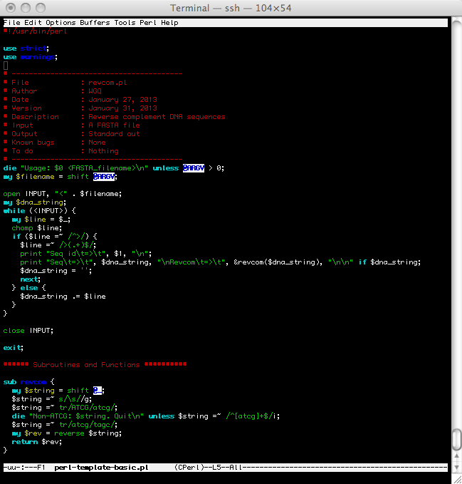
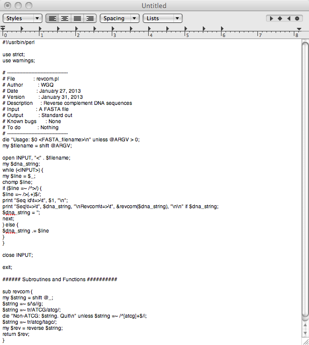
Useful Links
Unix Tutorials
- Oreilly Book for the virtues of command-line tools: Data Science at Command Line by Jeroen Janssens
- A very nice UNIX tutorial (you will only need up to, and including, tutorial 4).
- FOSSWire's Unix/Linux command reference (PDF). Of use to you: "File commands", "SSH", "Searching" and "Shortcuts".
Perl Help
- Professor Stewart Weiss has taught CSCI132, a UNIX and Perl class. His slides go into much greater detail and are an invaluable resource. They can be found on his course page here.
- Perl documentation at perldoc.perl.org. Besides that, running the perldoc command before either a function (with the -f option ie, perldoc -f substr) or a perl module (ie, perldoc Bio::Seq) can get you similar results without having to leave the terminal.
Regular Expression
Bioperl
- BioPerl's HOWTOs page.
- BioPerl-live developer documentation. (We use bioperl-live in class.)
- Yozen's tutorial on installing bioperl-live on your own Mac OS X machine. (Let me know if there are any issues!).
- A small table showing some methods for BioPerl modules with usage and return values.
SQL
- SQL Primer, written by Yozen.
R Project
- Install location and instructions for Windows
- Install location and instructions for Mac OS X
- Install R-Studio
- For users of Ubuntu/Debian:
sudo apt-get install r-base-core
© Weigang Qiu, Hunter College, Last Update ~~